\(\newcommand{L}[1]{\| #1 \|}\newcommand{VL}[1]{\L{ \vec{#1} }}\newcommand{R}[1]{\operatorname{Re}\,(#1)}\newcommand{I}[1]{\operatorname{Im}\, (#1)}\)

Find the arteries solution

>>> #: Our usual imports
>>> import numpy as np  # Python array library
>>> import matplotlib.pyplot as plt  # Python plotting library

The major arteries in a T1 MRI image often have high signal (white when displaying in gray-scale).

Our task is to see if we can pick out the courses of the vertebral, basilar and carotid arteries on this image.

The image is ds107_sub001_highres.nii. Download ds107_sub001_highres.nii to your working directory.

This time we are going to load the image using the nibabel library.

>>> #: Import nibabel
>>> import nibabel as nib

Try loading the image using nibabel, to make an image object. Use tab completion on nib. in IPython to see if you can fund the function you need. Go back to have a look at What is an image? if you are stuck.

>>> #- Use nibabel to load the image ds107_sub001_highres.nii
>>> #- img = ?
>>> img = nib.load('ds107_sub001_highres.nii')

Now get the image array data from the nibabel image object. Don’t forget to use tab completion on the image object if you can’t remember or don’t know the methods of the object.

>>> #- data = ?
>>> data = img.get_data()

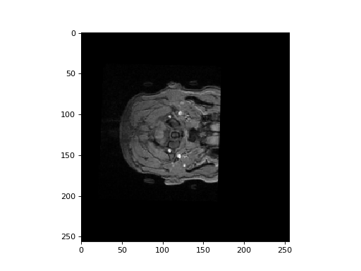
Try plotting a few slices over the third dimension to see whether you can see the arteries. For example, if data is your image array data, then you might plot the first slice over the third dimension, you might use:

plt.imshow(data[:, :, 0], cmap='gray')

>>> #- Plotting some slices over the third dimension
>>> plt.imshow(data[:, :, 30], cmap='gray')
<...>

(png, hires.png, pdf)

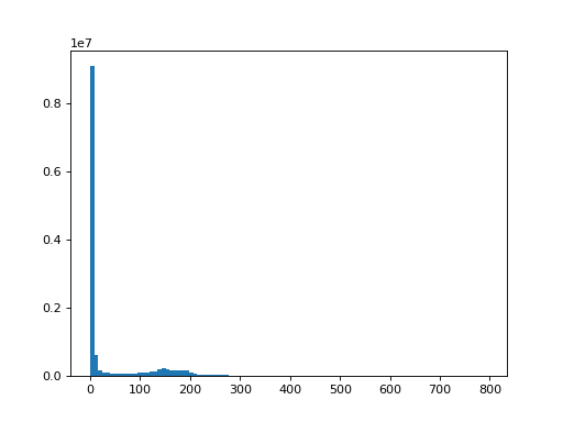
Now try looking for a good threshold so that you pick up only the very high signal in the brain. A good place to start is to use plt.hist to get an idea of the spread of values within the volume and within the slice.

>>> #- Here you might try plt.hist or something else to find a threshold
>>> data_1d = data.ravel()
>>> plt.hist(data_1d, bins=100)
(...)

(png, hires.png, pdf)

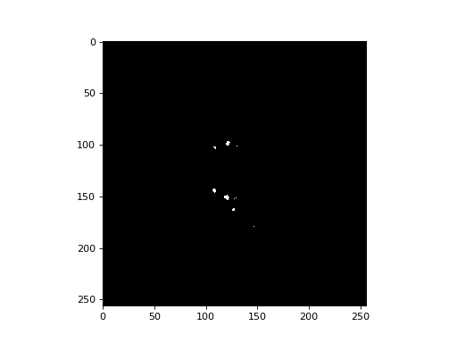
Try making a binarized image with your threshold and displaying slices with that. What structures are you picking up?

>>> #- Maybe display some slices from the data binarized with a threshold
>>> threshold = 300
>>> binarized_data = data > threshold
>>> plt.imshow(binarized_data[:, :, 30], cmap='gray')
<...>

(png, hires.png, pdf)

Now try taking a 3D subvolume out of the middle of the image. Take the approximate middle in all three axes. Use this to pick out a good subvolume of the image that still contains the big arteries.

>>> #- Create a smaller 3D subvolume from the image data that still
>>> #- contains the arteries
>>> subvolume = data[90:-90, 90:-90, 10:130]

Try binarizing the subvolume with some thresholds to see whether you can pick out the arteries without much other stuff. Hint - you might consider using np.percentile or plt.hist to find a good threshold.

>>> #- Try a few plots of binarized slices and other stuff to find a good
>>> #- threshold
>>> pct_99 = np.percentile(subvolume, 99)
>>> binarized_subvolume = subvolume > pct_99
>>> plt.imshow(binarized_subvolume[:, :, 20], cmap='gray')
<...>

(png, hires.png, pdf)

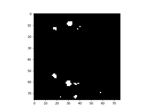
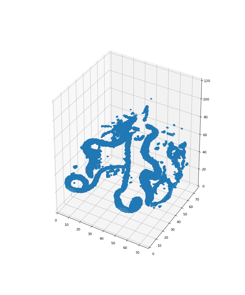
If you have a good threshold and a good binarized subset, see if you can see the arterial structure using the following fancy function to plot the binarized image with a 3D rendering. To use this function, you will need to install the scikit-image toolbox. First see if scikit-image is installed with the command import skimage from the Python / IPython console. If this gives you an ImportError, then open a new terminal window and install scikit-image with:

pip3 install --user scikit-image

Careful – do not run this pip3 install command from Python / IPython, but from the terminal command window.

When you have done the scikit-image install, uncomment this code:

>>> #: Uncomment the next line after installing scikit-image
>>> # from skimage import measure

With that import done, here is the fancy function to display your subvolume in 3D:

>>> #: This function uses matplotlib 3D plotting and sckit-image for
>>> # rendering
>>> from mpl_toolkits.mplot3d.art3d import Poly3DCollection
>>>
>>> def binarized_surface(binary_array):
...     """ Do a 3D plot of the surfaces in a binarized image
...
...     The function does the plotting with scikit-image and some fancy
...     commands that we don't need to worry about at the moment.
...     """
...     # Here we use the scikit-image "measure" function
...     verts, faces, norms, vals = mcubes(binary_array, 0)
...     fig = plt.figure(figsize=(10, 12))
...     ax = fig.add_subplot(111, projection='3d')
...
...     # Fancy indexing: `verts[faces]` to generate a collection of triangles
...     mesh = Poly3DCollection(verts[faces], linewidths=0, alpha=0.5)
...     ax.add_collection3d(mesh)
...     ax.set_xlim(0, binary_array.shape[0])
...     ax.set_ylim(0, binary_array.shape[1])
...     ax.set_zlim(0, binary_array.shape[2])

For example, let’s say you have a binarized subvolume of the original data called binarized_subvolume. You could do a 3D rendering of this binary image with:

binarized_surface(binarized_subvolume)

>>> binarized_surface(binarized_subvolume)

(png, hires.png, pdf)