\(\newcommand{L}[1]{\| #1 \|}\newcommand{VL}[1]{\L{ \vec{#1} }}\newcommand{R}[1]{\operatorname{Re}\,(#1)}\newcommand{I}[1]{\operatorname{Im}\, (#1)}\)

Convolving with the hemodyamic response function

Start with our usual imports:

>>> import numpy as np
>>> import matplotlib.pyplot as plt

Using scipy

Scipy is a large library of scientific routines that builds on top of numpy.

You can think of numpy as being a subset of MATLAB, and numpy + scipy as being as being roughly equivalent to MATLAB plus the MATLAB toolboxes.

Scipy has many sub-packages, for doing things like reading MATLAB .mat files (scipy.io) or working with sparse matrices (scipy.sparse). We are going to be using the functions and objects for working with statistical distributions in scipy.stats:

>>> import scipy.stats

scipy.stats contains objects for working with many different distributions. We are going to be working with scipy.stats.gamma, which implements the gamma distribution.

>>> from scipy.stats import gamma

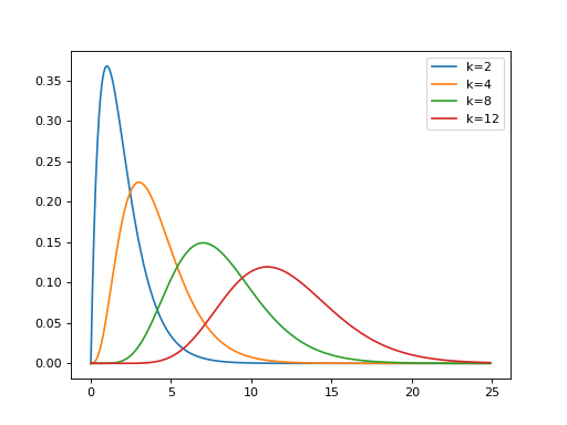
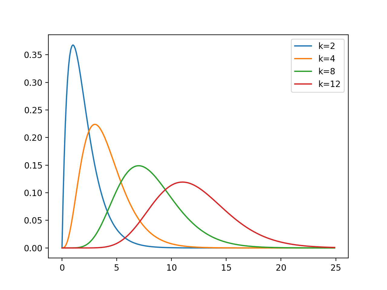
In particular we are interested in the probability density function (PDF) of the gamma distribution.

Because this is a function, we need to pass it an array of values at which it will evaluate.

We can also pass various parameters which change the shape, location and width of the gamma PDF. The most important is the first parameter (after the input array) known as the shape parameter (\(k\) in the wikipedia page on gamma distributions).

First we chose some x values at which to sample from the gamma PDF:

>>> x = np.arange(0, 25, 0.1)

Next we plot the gamma PDF for shape values of 2, 4, 8, 12.

>>> plt.plot(x, gamma.pdf(x, 2), label='k=2')
[...]
>>> plt.plot(x, gamma.pdf(x, 4), label='k=4')
[...]
>>> plt.plot(x, gamma.pdf(x, 8), label='k=8')
[...]
>>> plt.plot(x, gamma.pdf(x, 12), label='k=12')
[...]
>>> plt.legend()
<...>

(png, hires.png, pdf)

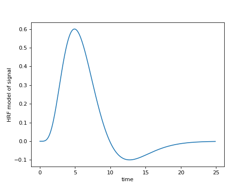
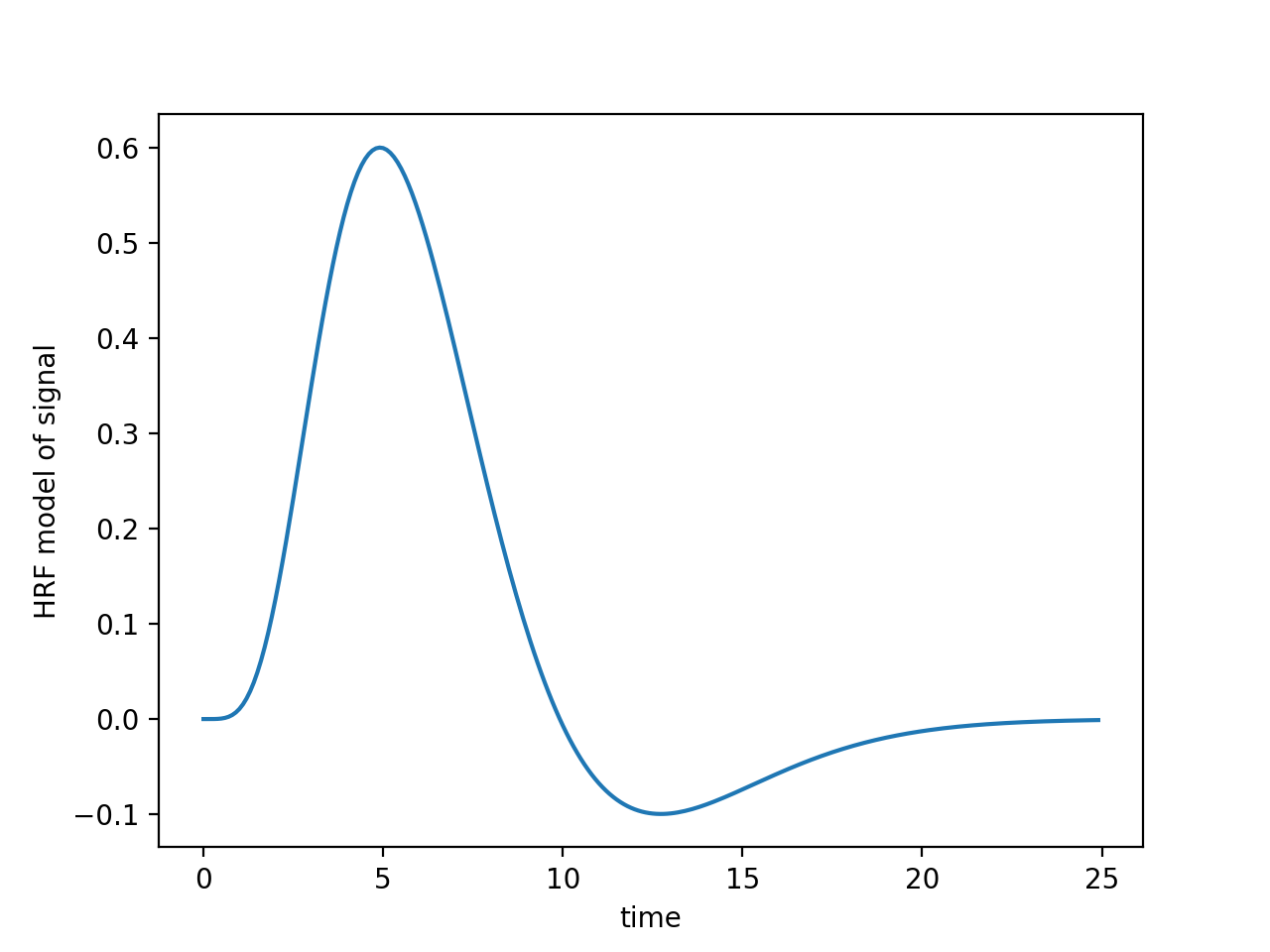
Constructing a hemodynamic response function

We can use these gamma functions to construct a continuous function that is close to the hemodynamic response we observe for a single brief event in the brain.

Our function will accept an array that gives the times we want to calculate the HRF for, and returns the values of the HRF for those times. We will assume that the true HRF starts at zero, and gets to zero sometime before 35 seconds.

We’re going to try using the sum of two gamma distribution probability density functions.

Here is one example of such a function:

>>> def hrf(times):
...     """ Return values for HRF at given times """
...     # Gamma pdf for the peak
...     peak_values = gamma.pdf(times, 6)
...     # Gamma pdf for the undershoot
...     undershoot_values = gamma.pdf(times, 12)
...     # Combine them
...     values = peak_values - 0.35 * undershoot_values
...     # Scale max to 0.6
...     return values / np.max(values) * 0.6

>>> plt.plot(x, hrf(x))
[...]
>>> plt.xlabel('time')
<...>
>>> plt.ylabel('HRF model of signal')
<...>

(png, hires.png, pdf)

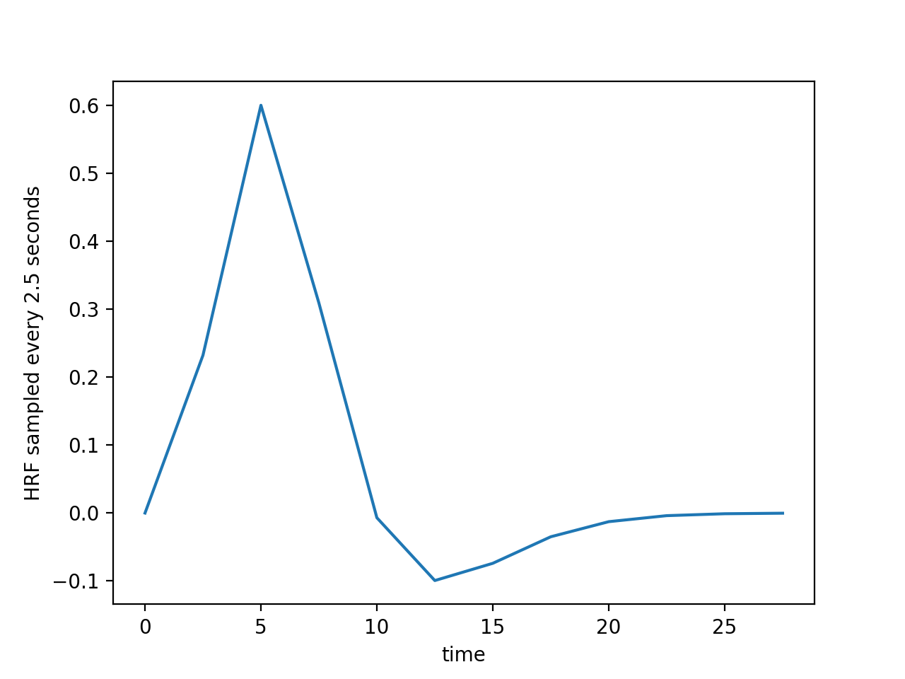
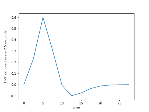
We can sample from the function, to get the estimates at the times of our TRs. Remember, the TR is 2.5 for our example data, meaning the scans were 2.5 seconds apart.

>>> TR = 2.5
>>> tr_times = np.arange(0, 30, TR)
>>> hrf_at_trs = hrf(tr_times)
>>> len(hrf_at_trs)
12
>>> plt.plot(tr_times, hrf_at_trs)
[...]
>>> plt.xlabel('time')
<...>
>>> plt.ylabel('HRF sampled every 2.5 seconds')
<...>

(png, hires.png, pdf)

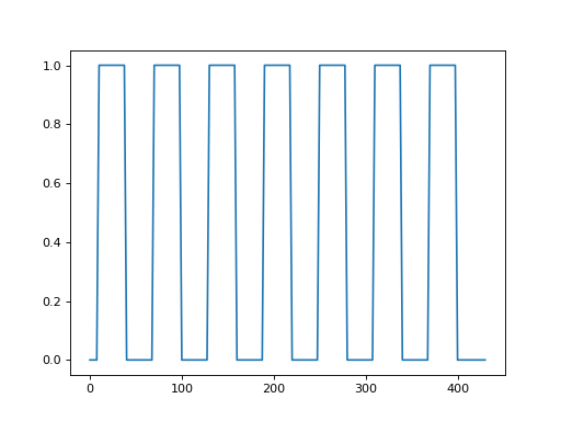
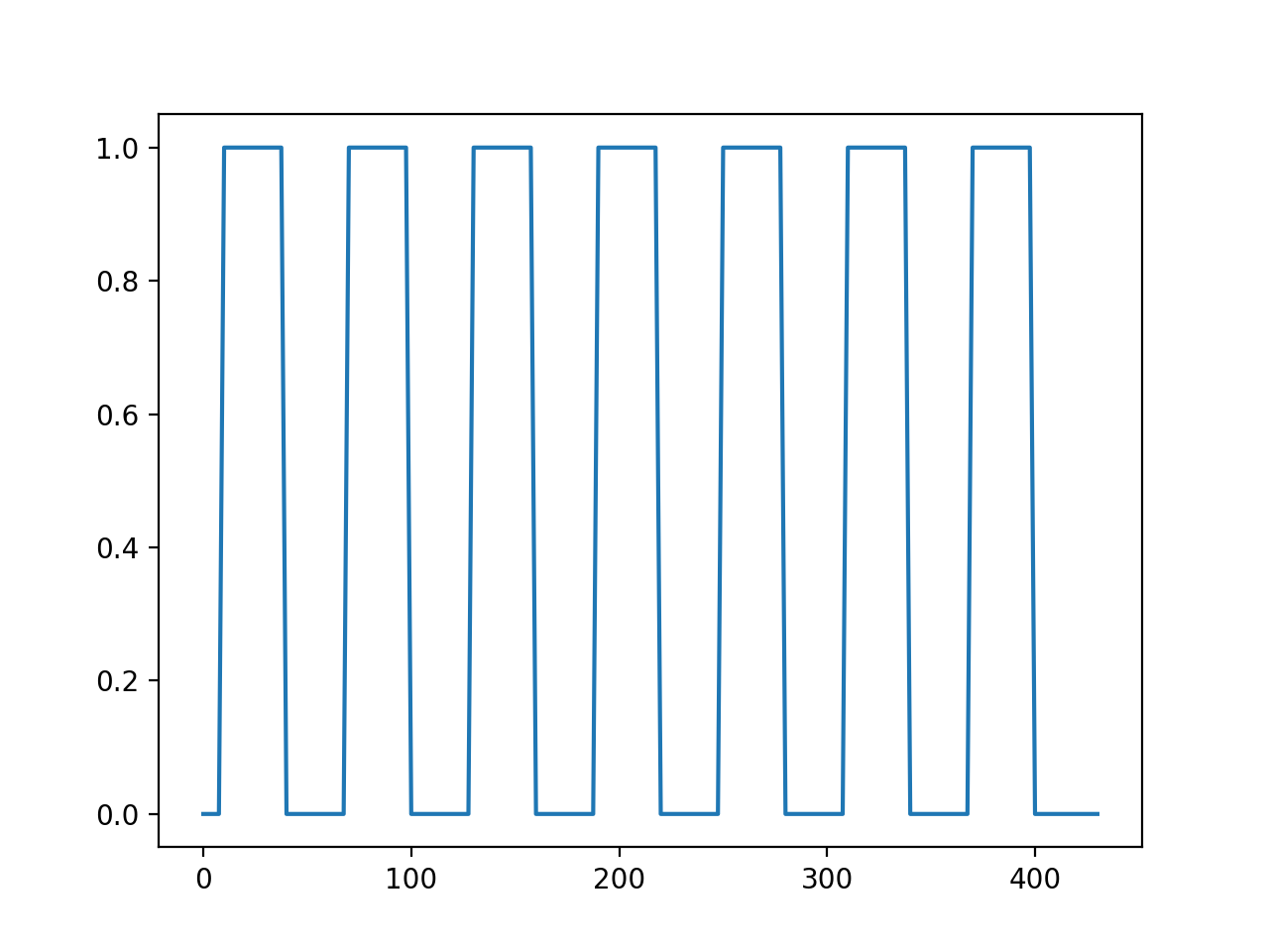
We can use this to convolve our neural (on-off) prediction. This will give us a hemodynamic prediction, under the linear-time-invariant assumptions of the convolution. Download stimuli.py if you don’t have it already.

>>> from stimuli import events2neural
>>> n_vols = 173
>>> neural_prediction = events2neural('ds114_sub009_t2r1_cond.txt',
...                                   TR, n_vols)
>>> all_tr_times = np.arange(173) * TR
>>> plt.plot(all_tr_times, neural_prediction)
[...]

(png, hires.png, pdf)

When we convolve, the output is length N + M-1, where N is the number of values in the vector we convolved, and M is the length of the convolution kernel (hrf_at_trs in our case). For a reminder of why this is, see the tutorial on convolution.

>>> convolved = np.convolve(neural_prediction, hrf_at_trs)
>>> N = len(neural_prediction)  # M == n_vols == 173
>>> M = len(hrf_at_trs)  # M == 12
>>> len(convolved) == N + M - 1
True

This is because of the HRF convolution kernel falling off the end of the input vector. The value at index 172 in the new vector refers to time 172 * 2.5 = 430.0 seconds, and value at index 173 refers to time 432.5 seconds, which is just after the end of the scanning run. To retain only the values in the new hemodynamic vector that refer to times up to (and including) 430s, we can just drop the last len(hrf_at_trs) - 1 == M - 1 values:

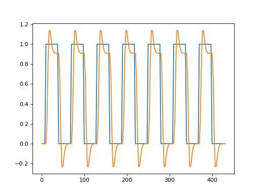
>>> n_to_remove = len(hrf_at_trs) - 1
>>> convolved = convolved[:-n_to_remove]

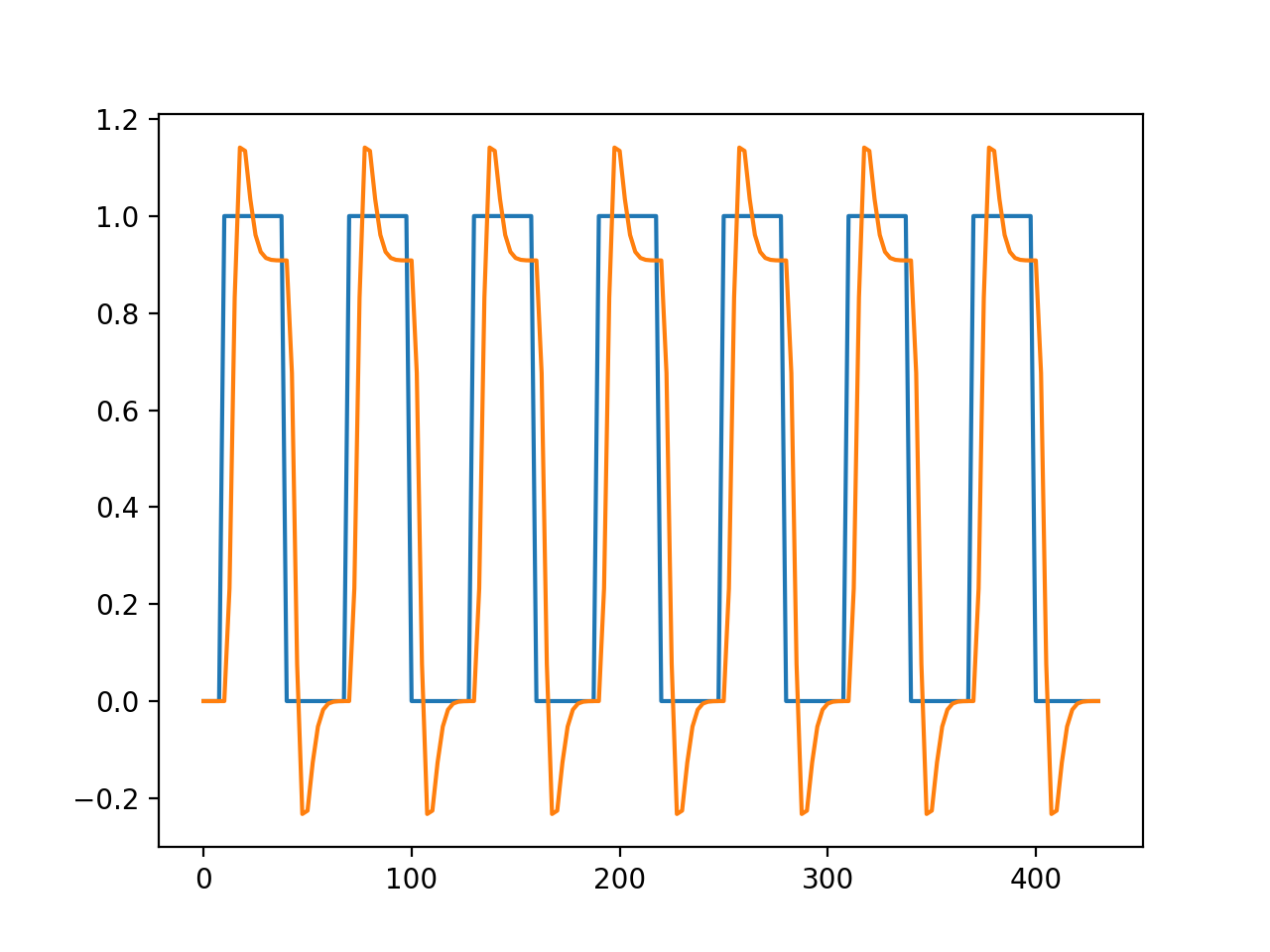
>>> plt.plot(all_tr_times, neural_prediction)
[...]
>>> plt.plot(all_tr_times, convolved)
[...]

(png, hires.png, pdf)

For our future use, let us save our convolved time course to a numpy text file:

>>> # Save the convolved time course to 6 decimal point precision
>>> np.savetxt('ds114_sub009_t2r1_conv.txt', convolved, fmt='%2.6f')
>>> back = np.loadtxt('ds114_sub009_t2r1_conv.txt')
>>> # Check written data is within 0.000001 of original
>>> np.allclose(convolved, back, atol=1e-6)
True