\(\newcommand{L}[1]{\| #1 \|}\newcommand{VL}[1]{\L{ \vec{#1} }}\newcommand{R}[1]{\operatorname{Re}\,(#1)}\newcommand{I}[1]{\operatorname{Im}\, (#1)}\)
Correlation per voxel, in 2D
In this exercise, we will take each voxel time course in the brain, and calculate a correlation between the task-on / task-off vector and the voxel time course. We then make a new 3D volume that contains correlation values for each voxel.
>>> #: Standard imports
>>> import numpy as np
>>> import matplotlib.pyplot as plt
>>> import nibabel as nib
Import the events2neural function from the stimuli.py module:
>>> #- import events2neural from stimuli module
>>> from stimuli import events2neural
If you don’t have it already, download the ds114_sub009_t2r1.nii
image. Load it with nibabel.
>>> #- Load the ds114_sub009_t2r1.nii image
>>> img = nib.load('ds114_sub009_t2r1.nii')
>>> #- Get the number of volumes in ds114_sub009_t2r1.nii
>>> n_trs = img.shape[-1]
The TR (time between scans) is 2.5 seconds.
>>> #: TR
>>> TR = 2.5
Call the events2neural function to give you a time course that is 1 for
the volumes during the task (thinking of verbs) and 0 for the volumes during
rest.
>>> #- Call events2neural to give on-off values for each volume
>>> time_course = events2neural('ds114_sub009_t2r1_cond.txt', 2.5, n_trs)
Using slicing, drop the first 4 volumes, and the corresponding on-off values:
>>> #- Drop the first 4 volumes, and the first 4 on-off values
>>> data = img.get_data()
>>> data = data[..., 4:]
>>> time_course = time_course[4:]
>>> #- Calculate the number of voxels (number of elements in one volume)
>>> n_voxels = np.prod(data.shape[:-1])
Reshape the 4D data to a 2D array shape (number of voxels, number of volumes).
>>> #- Reshape 4D array to 2D array n_voxels by n_volumes
>>> data_2d = np.reshape(data, (n_voxels, data.shape[-1]))
>>> #- Make a 1D array of size (n_voxels,) to hold the correlation values
>>> correlations_1d = np.zeros((n_voxels,))
If you finished the Pearson 1D and 2D function exercise exercise, you can use your
pearson_2d routine for calculating Pearson correlations across a 2D array.
Otherwise, loop over all voxels, calculate the correlation coefficient with
time_course at this voxel, and fill in the corresponding entry in your 1D
array.
>>> #- Loop over voxels filling in correlation at this voxel
>>> for i in range(n_voxels):
...     correlations_1d[i] = np.corrcoef(time_course, data_2d[i, :])[0, 1]
>>> #- Or (much faster) use pearson_2d function
>>> from pearson import pearson_2d
>>> correlations_1d = pearson_2d(time_course, data_2d.T)
Reshape the correlations 1D array back to a 3D array, using the original 3D shape.
>>> #- Reshape the correlations array back to 3D
>>> correlations = np.reshape(correlations_1d, data.shape[:-1])
Test that your brain-at-a-time correlation image gives the same answer when
you run the correlation on a single voxel time course. Select an example
voxel – say data[42, 32, 19] – and check that this gives the same
answer as you found for the matching voxel in your correlations 3D array:
>>> #- Check you get the same answer when selecting a voxel time course
>>> #- and running the correlation on that time course.  One example voxel
>>> #- could be the voxel at array coordinate [42, 32, 19]
>>> voxel_time_course = data[42, 32, 19]
>>> single_cc = np.corrcoef(voxel_time_course, time_course)[0, 1]
>>> assert np.allclose(correlations[42, 32, 19], single_cc)
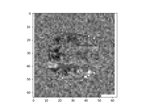
Plot the middle slice (plane) of the third axis from the correlations array. Look for any voxels with a high task correlation in the frontal lobe:
>>> #- Plot the middle slice of the third axis from the correlations array
>>> plt.imshow(correlations[:, :, 14], cmap='gray')
<...>