\(\newcommand{L}[1]{\| #1 \|}\newcommand{VL}[1]{\L{ \vec{#1} }}\newcommand{R}[1]{\operatorname{Re}\,(#1)}\newcommand{I}[1]{\operatorname{Im}\, (#1)}\)
Working with four dimensional images, masks and functions
>>> #: Our usual imports
>>> import numpy as np  # the Python array package
>>> import matplotlib.pyplot as plt  # the Python plotting package
Reading text files
We’ve been reading values from text files in the exercises.
Here is some revision on how to do that, going from the crude to the elegant way.
I first write a little text file out to disk:
>>> numbers = [1.2, 2.3, 3.4, 4.5]
>>> fobj = open('some_numbers.txt', 'wt')
>>> for number in numbers:
...     # String version of number, plus end-of-line character
...     fobj.write(str(number) + '\n')
4
4
4
4
>>> fobj.close()
Now I read it back again. First, I will read the all the lines in one shot, returning a list of strings:
>>> fobj = open('some_numbers.txt', 'rt')
>>> lines = fobj.readlines()
>>> len(lines)
4
>>> lines[0]
'1.2\n'
Next I will read the file, but converting each number to a float:
>>> fobj = open('some_numbers.txt', 'rt')
>>> numbers_again = []
>>> for line in fobj.readlines():
...     numbers_again.append(float(line))
>>> numbers_again
[1.2, 2.3, 3.4, 4.5]
In fact we can do this even more simply by using np.loadtxt:
>>> np.loadtxt('some_numbers.txt')
array([ 1.2,  2.3,  3.4,  4.5])
Loading data with nibabel
Nibabel allows us to load images. First we need to import the nibabel
library:
>>> import nibabel as nib
I am going to load the image with filename ds114_sub009_t2r1.nii.
Download the file from the link to type along.
First I load the image, to give me an “image” object:
>>> img = nib.load('ds114_sub009_t2r1.nii')
>>> type(img)
<class 'nibabel.nifti1.Nifti1Image'>
You can explore the image object with img. followed by TAB at the IPython
prompt.
Because images can have large arrays, nibabel does not load the image array
when you load the image, in order to save time and memory. The best way to
get the image array data is with the get_data() method.
>>> data = img.get_data()
>>> type(data)
<class 'numpy.core.memmap.memmap'>
The memmap is a special type of array that saves memory, but otherwise
behaves the same as any other numpy array.
I recommend you disable the use of the ‘memmap’ special arrays by using the
mmap keyword argument when you load the image.
>>> img = nib.load('ds114_sub009_t2r1.nii', mmap=False)
In this case you will get a normal array from get_data
>>> data = img.get_data()
>>> type(data)
<class 'numpy.ndarray'>
Four dimensional arrays - space + time
The image we have just loaded is a four-dimensional image, with a four-dimensional array:
>>> data.shape
(64, 64, 30, 173)
The first three axes represent three dimensional space. The last axis represents time. Here the last (time) axis has length 173. This means that, for each of these 173 elements, there is one whole three dimensional image. We often call the three-dimensional images volumes. So we could say that this 4D image contains 173 volumes.
We have previously been taking slices over the third axis of a three-dimensional image. We can now take slices over the fourth axis of this four-dimensional image:
>>> # A slice over the final (time) axis
>>> first_vol = data[:, :, :, 0]
This slice selects the first three-dimensional volume (3D image) from the 4D array:
>>> first_vol.shape
(64, 64, 30)
You can use the ellipsis ... when slicing an array. The ellipsis is a
short cut for “everything on the previous axes”. For example, these two have
exactly the same meaning:
>>> first_vol = data[:, :, :, 0]
>>> first_vol_again = data[..., 0]  # Using the ellipsis
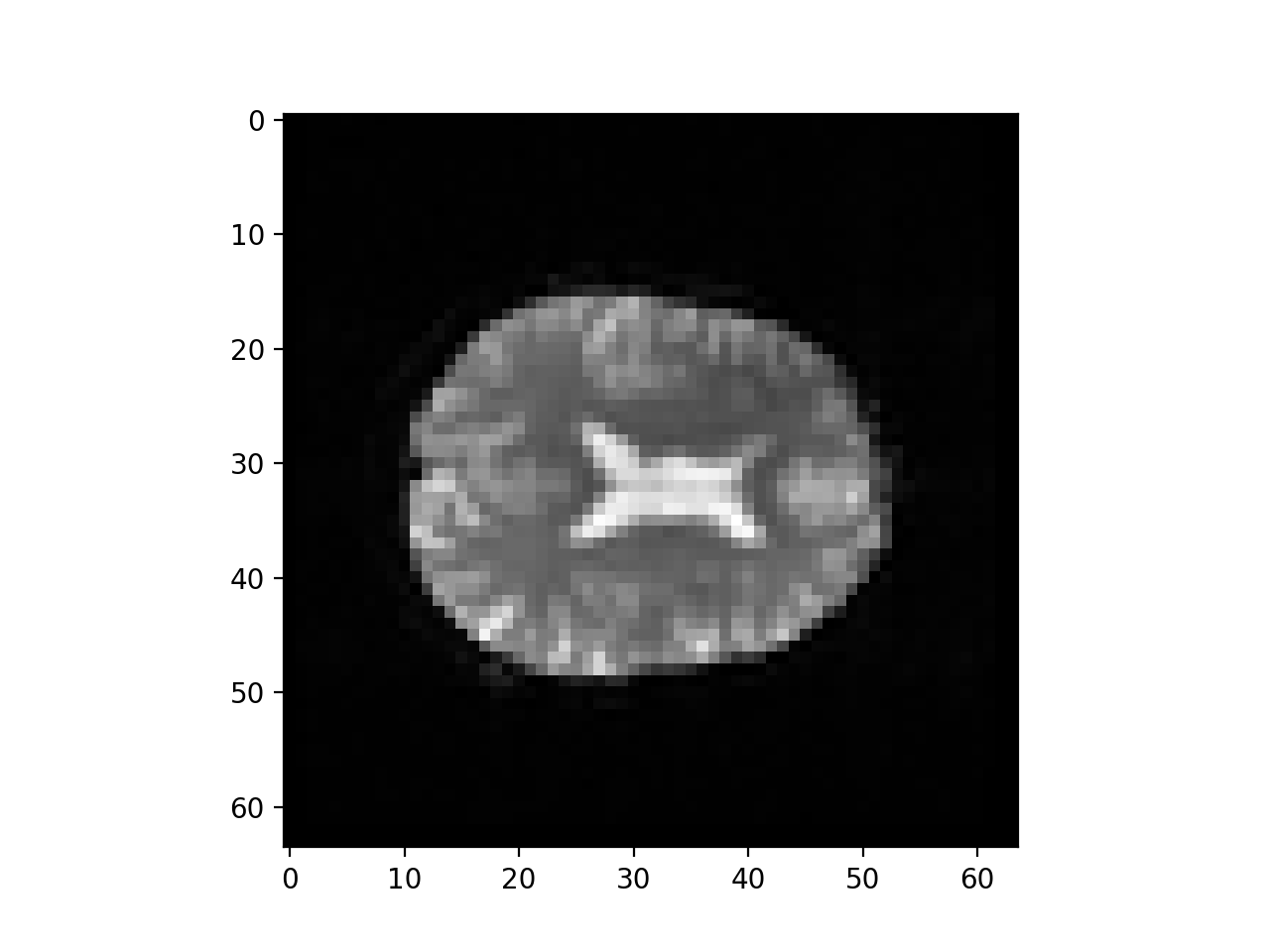
first_vol is a 3D image just like the 3D images you have already seen:
>>> # A slice over the third dimension
>>> plt.imshow(first_vol[:, :, 14], cmap='gray')
<...>

Numpy operations work on the whole array by default
Numpy operatons like min, and max and std operate on the whole
numpy array by default, ignoring any array shape. For example, here is the
maximum value for the whole 4D array:
>>> np.max(data)
6793
This is exactly the same as:
>>> # maximum when flattening the array to 1 dimension
>>> np.max(data.ravel())
6793
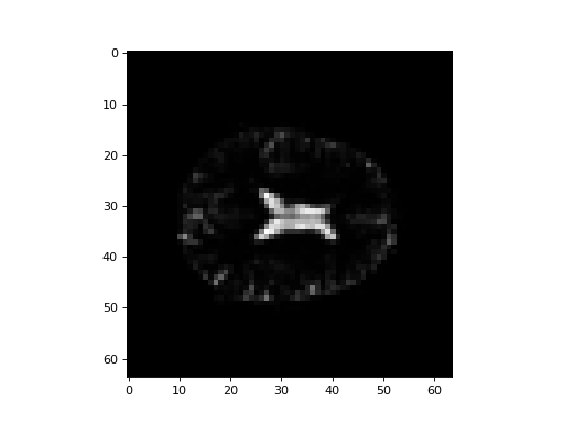
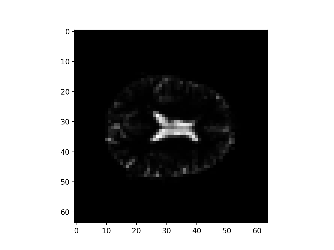
You can ask numpy to operate over particular axes instead of operating over the whole array. For example, this will generate a 3D image, where each array value is the variance over the 173 values at that 3D position (the variance across time):
>>> # variance across the final (time) axis
>>> var_vol = np.var(data, axis=3)
>>> plt.imshow(var_vol[:, :, 14], cmap='gray')
<...>

Indexing with boolean arrays
See the scipy lectures notes on the numpy array object.
Let’s say we have an array like this:
>>> arr = np.array([[0, 1, 3, 0], [5, 2, 0, 1]])
>>> arr
array([[0, 1, 3, 0],
       [5, 2, 0, 1]])
We can get a True / False (boolean) array to tell us whether these values are above some threshold:
>>> tf_array = arr > 2
>>> tf_array
array([[False, False,  True, False],
       [ True, False, False, False]], dtype=bool)
We can use this boolean array to index into the original array (or any array
with a suitable shape). This will select only the elements where the boolean
array is True. The returned array may well have selected only a few
members from any particular row or column or (in general) higher axis, so if
the mask has the same number of dimensions as the array being indexed, the
returned array is always one-dimensional to reflect the loss of shape:
>>> selected_elements = arr[tf_array]
>>> selected_elements
array([3, 5])
>>> selected_elements.shape
(2,)
We can use this to select values in our image as well. For example, if we
wanted to select only values less than 10 in first_vol:
>>> tf_lt_10 = first_vol < 10
>>> vals_lt_10 = first_vol[tf_lt_10]
>>> np.unique(vals_lt_10)
array([0, 1, 2, 3, 4, 5, 6, 7, 8, 9], dtype=int16)
Defining functions
See Brisk introduction to Python.
A function takes input arguments, transforms them, and returns the output. For example, the following function adds two numbers:
>>> def add(a, b):
...     return a + b
Functions can also return multiple values, for example:
>>> def weather():
...     return 'hot', 'north-east', 78
...
>>> sun, wind, temp = weather()
>>>
>>> print('Sun:', sun)
Sun: hot
>>> print('Window:', wind)
Window: north-east
>>> print('Temperature:', temp)
Temperature: 78