\(\newcommand{L}[1]{\| #1 \|}\newcommand{VL}[1]{\L{ \vec{#1} }}\newcommand{R}[1]{\operatorname{Re}\,(#1)}\newcommand{I}[1]{\operatorname{Im}\, (#1)}\)
Making our own hemodynamic response function
- For code template see:
make_an_hrf_code.py; - For solution see: Making our own hemodynamic response function.
>>> #: Import array and plotting libraries.
>>> import numpy as np
>>> import matplotlib.pyplot as plt
>>> # Print arrays to 4 decimal places
>>> np.set_printoptions(precision=4, suppress=True)
The file mt_hrf_estimates.txt contains the estimated FMRI signal
from voxels in the MT motion area at 0, 2, 4, …, 28 seconds after a brief
moving visual stimulus (see:
http://nipy.org/nitime/examples/event_related_fmri.html).
Here are the first four rows. The numbers are in exponential floating point format:
1.394086932967517900e-01
3.938585701431884800e-01
5.012927230566770476e-01
5.676763716149294536e-01
Read the values from the file into an array mt_hrf_estimates. Make a
new array mt_hrf_times with the times of acquisition (0, 2, …).
Plot them together to see the HRF estimate at these times:
>>> #- Load the estimated values from the text file into an array
>>> #- Make an array of corresponding times
>>> #- Plot signal by time
We want to make a hemodynamic response function that matches this shape.
Our function will accept an array that gives the times we want to calculate the HRF for, and returns the values of the HRF for those times. We will assume that the true HRF starts at zero, and gets to zero sometime before 35 seconds.
Like SPM, I’m going to try using the sum of two gamma distribution probability density functions.
>>> #: import the gamma density function
>>> from scipy.stats import gamma
Here’s my first shot:
>>> #: my attempt - you can do better than this
>>> def not_great_hrf(times):
...     """ Return values for HRF at given times """
...     # Gamma pdf for the peak
...     peak_values = gamma.pdf(times, 6)
...     # Gamma pdf for the undershoot
...     undershoot_values = gamma.pdf(times, 12)
...     # Combine them
...     values = peak_values - 0.35 * undershoot_values
...     # Scale max to 0.6
...     return values / np.max(values) * 0.6
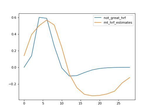
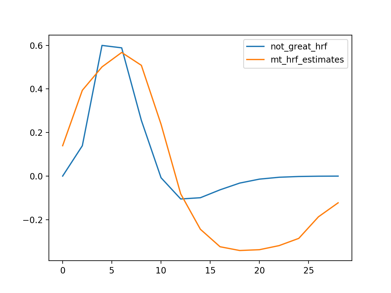
>>> #: plot the data against my estimate
>>> plt.plot(mt_hrf_times, not_great_hrf(mt_hrf_times), label='not_great_hrf')
[...]
>>> plt.plot(mt_hrf_times, mt_hrf_estimates, label='mt_hrf_estimates')
[...]
>>> plt.legend()
<...>

Now see if you can make a better function by playing with the Gamma
distribution PDF parameter, and the mix of the two gamma distribution
functions. Call your function mt_hrf
>>> #- Your "mt_hrf" function here
>>> #- Plot your function against the mt_hrf_estimates data to test
For extra points - other than looking at these plots, how would you convince me your function is better than mine?
>>> #- Evidence that your function is better than mine?