\(\newcommand{L}[1]{\| #1 \|}\newcommand{VL}[1]{\L{ \vec{#1} }}\newcommand{R}[1]{\operatorname{Re}\,(#1)}\newcommand{I}[1]{\operatorname{Im}\, (#1)}\)

Estimation for many voxels at the same time

We often want to fit the same design to many different voxels.

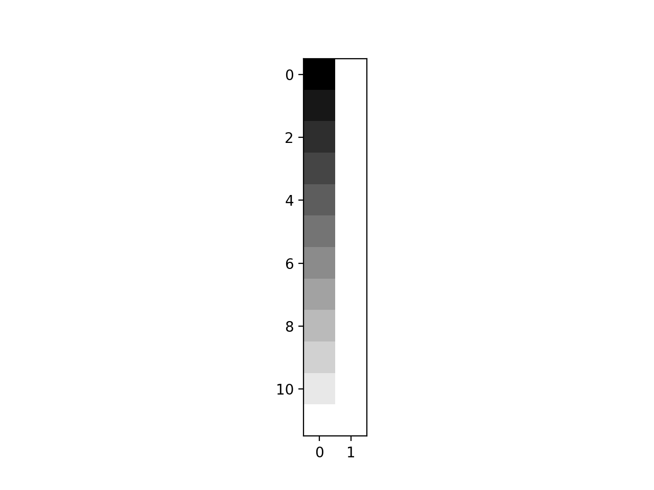
Let’s make a design with a linear trend and a constant term:

>>> import numpy as np
>>> import matplotlib.pyplot as plt
>>> # Print arrays to 4 decimal places
>>> np.set_printoptions(precision=4)

>>> X = np.ones((12, 2))
>>> X[:, 0] = np.linspace(-1, 1, 12)
>>> plt.imshow(X, interpolation='nearest', cmap='gray')
<...>

(png, hires.png, pdf)

To fit this design to any data, we take the pseudoinverse:

>>> import numpy.linalg as npl
>>> piX = npl.pinv(X)
>>> piX.shape
(2, 12)

Now let’s make some data to fit to. We will draw some somples from the standar normal distribution using numpy.random. We use numpy.random.seed to make sure the random numbers are predictable:

>>> np.random.seed(42)
>>> y_0 = np.random.normal(size=12)
>>> beta_0 = piX.dot(y_0)
>>> beta_0
array([-0.373,  0.296])

We can fit this same design to another set of data:

>>> y_1 = np.random.normal(size=12)
>>> beta_1 = piX.dot(y_1)
>>> beta_1
array([ 0.3405, -0.5912])

Now the trick. Because of the way that matrix multiplication works, we can fit to these two sets of data with the same call to dot:

>>> Y = np.vstack((y_0, y_1)).T
>>> betas = piX.dot(Y)
>>> betas
array([[-0.373 ,  0.3405],
       [ 0.296 , -0.5912]])

Of course this is true for any number of columns of Y.