\(\newcommand{L}[1]{\| #1 \|}\newcommand{VL}[1]{\L{ \vec{#1} }}\newcommand{R}[1]{\operatorname{Re}\,(#1)}\newcommand{I}[1]{\operatorname{Im}\, (#1)}\)
PCA exercise
>>> #: import common modules
>>> import numpy as np  # the Python array package
>>> import matplotlib.pyplot as plt  # the Python plotting package
>>> # Display array values to 6 digits of precision
>>> np.set_printoptions(precision=4, suppress=True)
>>> #: import numpy.linalg with a shorter name
>>> import numpy.linalg as npl
Download the image ds114_sub009_t2r1.nii if you don’t already have
it. Load it with nibabel. Get the data.
>>> #- Load the image 'ds114_sub009_t2r1.nii' with nibabel
>>> #- Get the data array from the image
>>> import nibabel as nib
>>> img = nib.load('ds114_sub009_t2r1.nii')
>>> data = img.get_data()
>>> data.shape
(64, 64, 30, 173)
We can think of the shape of the data as two parts - the first 3 values are the 3D shape of the individual volumes, and the last value is the number of volumes.
Put the 3D shape into a variable vol_shape and the number of volumes into
a variable n_vols:
>>> #- Make variables:
>>> #- 'vol_shape' for shape of volumes
>>> #- 'n_vols' for number of volumes
>>> vol_shape = data.shape[:-1]
>>> n_vols = data.shape[-1]
We are going to take the time axis as containing the “features”. We will take the voxels as being the “samples”. We start by taking the first two features (time points).
Slice the data array to make a new array that contains only the first two volumes:
>>> #- Slice the image data array to give array with only first two
>>> #- volumes
>>> first_two = data[..., :2]
>>> first_two.shape
(64, 64, 30, 2)
How many voxels are there in one volume? Put this number in a variable N:
>>> #- Set N to be the number of voxels in a volume
>>> N = np.prod(vol_shape)
Reshape the new two-volume data array to have a first dimension length N
and second dimension length 2. Each of the two columns corresponds to the
voxels for a whole volume.
>>> #- Reshape to 2D array with first dimension length N
>>> first_two = first_two.reshape((N, 2))
>>> first_two.shape
(122880, 2)
Take the transpose of this array to get a 2 by N array, ready for the PCA:
>>> #- Transpose to 2 by N array
>>> first_two = first_two.T
>>> first_two.shape
(2, 122880)
Calculate the mean across columns (row means). Put these means into a
variable row_means.
>>> #- Calculate the mean across columns
>>> row_means = np.mean(first_two, axis=1)
>>> row_means  # doctest: +SKIP
array([ 414.4011,  336.6994])
Expand the row_means vector out to a 2 by N array by using np.outer
and a vector of ones:
>>> #- Row means copied N times to become a 2 by N array
>>> row_means = np.outer(row_means, np.ones(N))
>>> row_means.shape
(2, 122880)
Subtract this expanded 2 by N means array from the 2 by N data matrix and put
the result into a variable X. Print the means across columns (row means)
to check they are now very close to 0:
>>> #- Subtract the means for each row, put the result into X
>>> #- Show the means over the columns, after the subtraction
>>> X = first_two - row_means
>>> np.mean(X, axis=1)  # doctest: +SKIP
array([-0.,  0.])
Plot the two rows against each other to get a feel for the variation.
Remember that each row in X is a volume, so you are plotting the signal
from the first volume against the corresponding signal for the second volume.
>>> #- Plot the signal in the first row against the signal in the second
>>> plt.plot(X[0], X[1], '+')
[...]

Time for the PCA.
We are going to use the unscaled covariance across time. This is given by
the matrix multiplication of X with its transpose. Calculate this:
>>> #- Calculate unscaled covariance matrix for X
>>> unscaled_covariance = X.dot(X.T)
>>> unscaled_covariance # doctest: +SKIP
array([[  8.0424e+10,   6.1264e+10],
      [  6.1264e+10,   4.9249e+10]])
Use SVD to get the U, S and VT matrices from the unscaled
covariance:
>>> #- Use SVD to return U, S, VT matrices from unscaled covariance
>>> U, S, VT = npl.svd(unscaled_covariance)
Confirm that the column vectors in U are both unit vectors. A unit vector
has vector length (vector norm) 1:
>>> #- Show that the columns in U each have vector length 1
>>> np.sum(U ** 2, axis=0)  # doctest: +SKIP
array([ 1.,  1.])
Confirm that the first column in U is orthogonal to the second:
>>> #- Confirm orthogonality of columns in U
>>> np.allclose(U[:, 0].dot(U[:, 1]), 0)
True
Confirm that the transpose of U is also the matrix inverse of U:
>>> #- Confirm tranpose of U is inverse of U
>>> np.allclose(np.eye(2), U.T.dot(U))
True
Show the total sum of squares in X. Confirm that the total sum of squares
in X is the same as the sum of the singular values in the S vector
from the SVD:
>>> #- Show the total sum of squares in X
>>> #- Is this (nearly) the same as the sum of the values in S?
>>> print(np.sum(X ** 2))  # doctest: +SKIP
129672885307.0
>>> print(np.sum(S))
129672885307.0
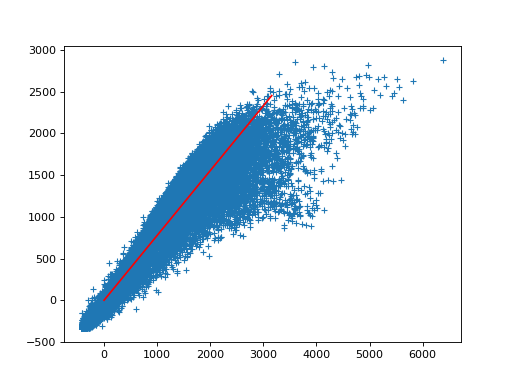
Plot the first row in X against the second row in X again. This
time add a line to the plot that corresponds to the first principal component.
You’ll have to scale this line (a unit vector) to make it long enough to see
on the axes of the plot. If the first principal component is flipped
(\(\vec{r}\) defines same line as \(-\vec{r}\)) you may need to scale
by a negative number for it to look nice on the plot:
>>> #- Plot the signal in the first row against the signal in the second
>>> #- Plot line corresponding to a scaled version of the first principal component
>>> #- (Scaling may need to be negative)
>>> plt.plot(X[0], X[1], '+')
[...]
>>> scaled_u = U[0, :] * -4000
>>> plt.plot([0, scaled_u[0]], [0, scaled_u[1]], 'r')
[...]
>>> scaled_u[0]
3157.9395737...
Remember the projection formula \(c = \hat{u} \cdot \vec{v}\).
We now need to calculate the scalar projections \(c\) for each component \(\hat{u}\) and each voxel (each \(\vec{v}\)).
This will give us a new output matrix of scalar projections \(C\) of shape
(2, N), where the rows give the scalar projections for one component, and
the columns give the coefficients for one voxel.
For example, C[0, 0] will be the result of U[0, :].dot(X[:, 0]), C[0,
1] will be the result of U[0, :].dot(X[:, 1]), and C[1, 0] will be the
result of U[:, 1].dot(X[:, 0]).
With that background, use matrix multiplication to calculate the scalar
projections C for projecting the data X onto the vectors in U:
>>> #- Calculate the scalar projections for projecting X onto the
>>> #- vectors in U.
>>> #- Put the result into a new array C.
>>> C = U.T.dot(first_two)
>>> C.shape
(2, 122880)
Remember that C - the matrix of scalar projections – has one column per
voxel. We can think of each row as corresponding to a volume where the volumes
are contained in: C[0] (first row of C) – scalar projections for
first principal component; C[1] (second row of C) – scalar projections
for second principal component.
Take the transpose of C and reshape the resulting first dimension (length
N) back to vol_shape - the original shape of the 3D volumes in the
data:
>>> #- Transpose C
>>> #- Reshape the first dimension of C to have the 3D shape of the
>>> #- original data volumes.
>>> C_vols = C.T.reshape(vol_shape + (2,))
>>> C_vols.shape
(64, 64, 30, 2)
Break this 4D array up into two volumes (volume for first component, volume for second component) using slicing:
>>> #- Break 4D array into two 3D volumes
>>> vol0 = C_vols[..., 0]
>>> vol1 = C_vols[..., 1]
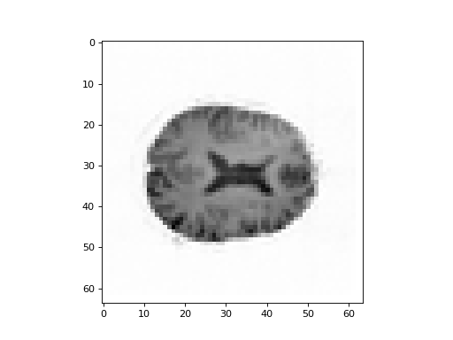
Show the middle plane (slice over the third dimension) from the volume of scalar projections for the first component:
>>> #- Show middle slice (over third dimension) from scalar projections
>>> #- for first component
>>> plt.imshow(vol0[:, :, 14], cmap='gray')
<...>
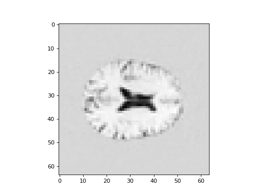
Show the middle plane (slice over the third dimension) from the volume of scalar projections for the second component:
>>> #- Show middle slice (over third dimension) from scalar projections
>>> #- for second component
>>> plt.imshow(vol1[:, :, 14], cmap='gray')
<...>
Now we are ready to do the same thing for all the time points, instead of just the first two.
Take the original array data matrix with n_vols volumes. Reshape to be
shape (N, nvols). Take the transpose to get an array shape (n_vols,
N):
>>> #- Reshape first dimension of whole image data array to N, and take
>>> #- transpose
>>> arr = data.reshape(N, n_vols).T
>>> arr.shape
(173, 122880)
Calculate the mean across columns (mean per volume). Expand this 1D shape
(173,) vector to an array shape (173, N), using np.outer and a
vector of ones. Subtract this array from the (173, N) data array to remove
the mean across columns (mean per volume). Call this mean-corrected variable
X:
>>> #- Calculate mean across columns
>>> #- Expand to (173, N) shape using np.outer
>>> #- Subtract from data array to remove mean over columns (row means)
>>> #- Put result into array X
>>> row_means = np.outer(np.mean(arr, axis=1), np.ones(N))
>>> X = arr - row_means
Get the unscaled covariance matrix of X:
>>> #- Calculate unscaled covariance matrix of X
>>> unscaled_covariance = X.dot(X.T)
>>> unscaled_covariance.shape
(173, 173)
Get U, S, VT outputs from the SVD of the unscaled covariance
>>> # Calculate U, S, VT with SVD on unscaled covariance matrix
>>> U, S, VT = npl.svd(unscaled_covariance)
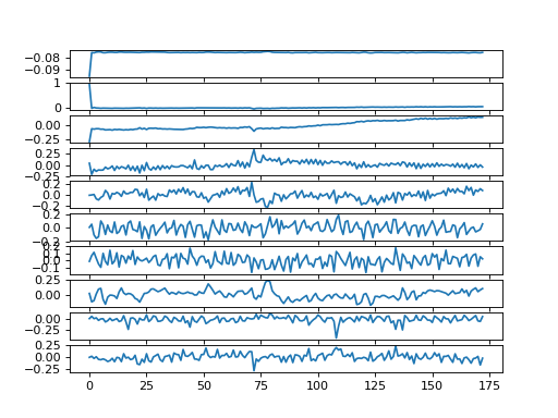
Use plt.subplots to make a column of 10 axes. Iterate over these axes,
plotting one principal component vector per axis. You should then have a plot
of each of the first 10 principal component vectors:
>>> #- Use subplots to make axes to plot first 10 principal component
>>> #- vectors
>>> #- Plot one component vector per sub-plot.
>>> fig, axes = plt.subplots(10, 1)
>>> for i, ax in enumerate(axes):
...     ax.plot(U[:, i])
[...]
Use U and matrix multiplication to calculate the scalar projection
coefficients for projecting the data X onto the principal components
U. Put the result into C:
>>> #- Calculate scalar projections for projecting X onto U
>>> #- Put results into array C.
>>> C = U.T.dot(X)
Remember, each row of C is a full volume of scalar projections, one row
per principal component.
Reconstruct these rows as volumes by taking the transpose of C and
reshaping the first dimension length N to the original three dimensions of
the original data volumes.
>>> #- Transpose C
>>> #- Reshape the first dimension of C to have the 3D shape of the
>>> #- original data volumes.
>>> C_vols = C.T.reshape(img.shape)
Take the first volume (corresponding to the first principal component) and display the middle plane (slicing over the third dimension):
>>> #- Show middle slice (over third dimension) of first principal
>>> #- component volume
>>> plt.imshow(C_vols[:, :, 14, 0], cmap='gray')
<...>
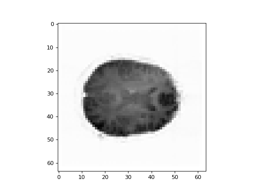
What does this first component show us?
Remember that the projections coefficients tell us how much of the component vector there is in the data, at each voxel. If the voxel has a high value it means there is a large amplitude of the component time-course at this voxel, and if the component is dark it means there is a large negative amplitude of the component time course.
Have a look again at the first component time course. How would a large positive or negative amplitude of the time course come about?
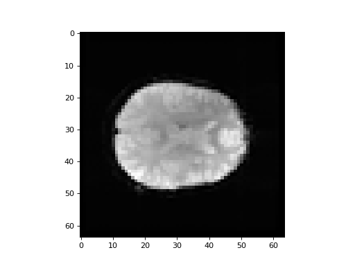
As a hint while you are thinking, get the mean over time from the image data (mean over the last axis), and show the middle plane (slicing over the third axis):
>>> #- Make the mean volume (mean over the last axis)
>>> #- Show the middle plane (slicing over the third axis)
>>> mean_vol = data.mean(axis=-1)
>>> plt.imshow(mean_vol[:, :, 14], cmap='gray')
<...>
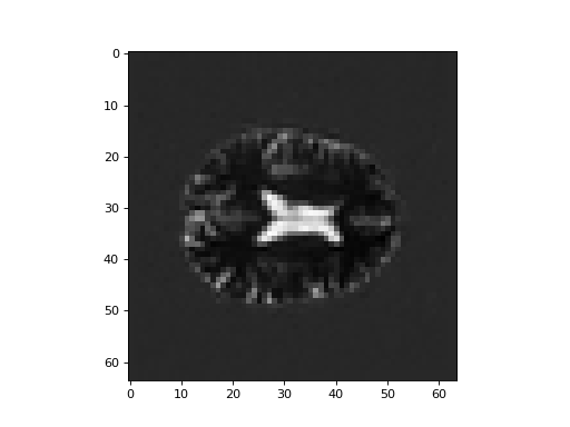
Display the middle plane (slicing over the third dimension) for the second principal component volume.
Looking at the principal component plot - what kind of changes over time does this principal component represent?
>>> #- Show middle plane (slice over third dimension) of second principal
>>> #- component volume
>>> plt.imshow(C_vols[:, :, 14, 1], cmap='gray')
<...>
Do the same for the third principal component volume:
>>> #- Show middle plane (slice over third dimension) of third principal
>>> #- component volume
>>> plt.imshow(C_vols[:, :, 14, 2], cmap='gray')
<...>
