\(\newcommand{L}[1]{\| #1 \|}\newcommand{VL}[1]{\L{ \vec{#1} }}\newcommand{R}[1]{\operatorname{Re}\,(#1)}\newcommand{I}[1]{\operatorname{Im}\, (#1)}\)
Slice timing exercise
See: slice timing correction for the background to this exercise.
>>> #: Import common modules
>>> import numpy as np  # the Python array package
>>> np.set_printoptions(precision=4, suppress=True)  # print to 4 DP
>>> import matplotlib.pyplot as plt  # the Python plotting package
>>> import nibabel as nib
>>> #: Set defaults for plotting
>>> plt.rcParams['image.cmap'] = 'gray'
>>> plt.rcParams['image.interpolation'] = 'nearest'
Load the image ds114_sub009_t2r1.nii with nibabel. Get the data:
>>> #: Load the image 'ds114_sub009_t2r1.nii' with nibabel
>>> # Get the data array from the image
>>> import nibabel as nib
>>> img = nib.load('ds114_sub009_t2r1.nii')
>>> data = img.get_data()
>>> data.shape
(64, 64, 30, 173)
As you remember, the first volume in this dataset is a lot different from the rest, and this will mess up our interpolation in time.
So, we need to remove the first volume from the data first, using slicing:
>>> #: Remove the first volume by slicing
>>> fixed_data = data[..., 1:]
>>> fixed_data.shape
(64, 64, 30, 172)
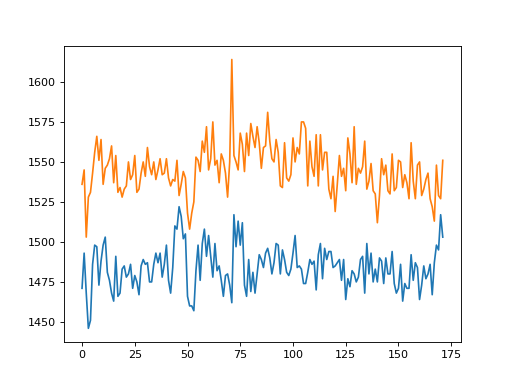
We start off with example time-courses from the first and second slice.
Use slicing to get a z slice 0 time series for an example voxel at voxel coordinates (23, 19, 0).
Do the same for a z slice 1 time series from (23, 19, 1).
Plot these time series against volume number on the same graph:
>>> #- Slice out time series for voxel (23, 19, 0)
>>> #- Slice out time series for voxel (23, 19, 1)
>>> #- Plot both these time series against volume number, on the same graph
>>> slice_0_ts = fixed_data[23, 19, 0, :]
>>> slice_1_ts = fixed_data[23, 19, 1, :]
>>> plt.plot(slice_0_ts)
[...]
>>> plt.plot(slice_1_ts)
[...]

The scanner collected slices for these data in an “ascending interleaved” order. That is, the scanner first collected z slice 0, then z slice 2, up to z slice 28. It then went back to collect z slice 1, 3, 5 up to z slice 29.
That means the scanner started collecting slice 0 in each volume, at the beginning of the volume.
The TR (time to collect one volume) is 2.5 seconds.
>>> #: The time between scans
>>> TR = 2.5
Make a time vector, length 172, that corresponds to the start time in seconds of each volume. This also gives the slice 0 start times.
>>> #- Make time vector containing start times in second of each volume,
>>> #- relative to start of first volume.
>>> #- Call this `slice_0_times`
>>> slice_0_times = np.arange(fixed_data.shape[-1]) * 2.5
>>> slice_0_times
array([   0. ,    2.5,    5. ,    7.5,   10. ,   12.5,   15. ,   17.5,
         20. ,   22.5,   25. ,   27.5,   30. ,   32.5,   35. ,   37.5,
         40. ,   42.5,   45. ,   47.5,   50. ,   52.5,   55. ,   57.5,
         60. ,   62.5,   65. ,   67.5,   70. ,   72.5,   75. ,   77.5,
         80. ,   82.5,   85. ,   87.5,   90. ,   92.5,   95. ,   97.5,
        100. ,  102.5,  105. ,  107.5,  110. ,  112.5,  115. ,  117.5,
        120. ,  122.5,  125. ,  127.5,  130. ,  132.5,  135. ,  137.5,
        140. ,  142.5,  145. ,  147.5,  150. ,  152.5,  155. ,  157.5,
        160. ,  162.5,  165. ,  167.5,  170. ,  172.5,  175. ,  177.5,
        180. ,  182.5,  185. ,  187.5,  190. ,  192.5,  195. ,  197.5,
        200. ,  202.5,  205. ,  207.5,  210. ,  212.5,  215. ,  217.5,
        220. ,  222.5,  225. ,  227.5,  230. ,  232.5,  235. ,  237.5,
        240. ,  242.5,  245. ,  247.5,  250. ,  252.5,  255. ,  257.5,
        260. ,  262.5,  265. ,  267.5,  270. ,  272.5,  275. ,  277.5,
        280. ,  282.5,  285. ,  287.5,  290. ,  292.5,  295. ,  297.5,
        300. ,  302.5,  305. ,  307.5,  310. ,  312.5,  315. ,  317.5,
        320. ,  322.5,  325. ,  327.5,  330. ,  332.5,  335. ,  337.5,
        340. ,  342.5,  345. ,  347.5,  350. ,  352.5,  355. ,  357.5,
        360. ,  362.5,  365. ,  367.5,  370. ,  372.5,  375. ,  377.5,
        380. ,  382.5,  385. ,  387.5,  390. ,  392.5,  395. ,  397.5,
        400. ,  402.5,  405. ,  407.5,  410. ,  412.5,  415. ,  417.5,
        420. ,  422.5,  425. ,  427.5])
The scanner starts to collect z slice 1 exactly half way through the volume (half way through the TR). Make a new vector that is the start time of acquisition of slice 1.
>>> #- Make time vector containing start times in seconds of z slice 1,
>>> #- relative to start of first volume.
>>> #- Call this `slice_1_times`
>>> slice_1_times = slice_0_times + 2.5 / 2
>>> slice_1_times
array([   1.25,    3.75,    6.25,    8.75,   11.25,   13.75,   16.25,
         18.75,   21.25,   23.75,   26.25,   28.75,   31.25,   33.75,
         36.25,   38.75,   41.25,   43.75,   46.25,   48.75,   51.25,
         53.75,   56.25,   58.75,   61.25,   63.75,   66.25,   68.75,
         71.25,   73.75,   76.25,   78.75,   81.25,   83.75,   86.25,
         88.75,   91.25,   93.75,   96.25,   98.75,  101.25,  103.75,
        106.25,  108.75,  111.25,  113.75,  116.25,  118.75,  121.25,
        123.75,  126.25,  128.75,  131.25,  133.75,  136.25,  138.75,
        141.25,  143.75,  146.25,  148.75,  151.25,  153.75,  156.25,
        158.75,  161.25,  163.75,  166.25,  168.75,  171.25,  173.75,
        176.25,  178.75,  181.25,  183.75,  186.25,  188.75,  191.25,
        193.75,  196.25,  198.75,  201.25,  203.75,  206.25,  208.75,
        211.25,  213.75,  216.25,  218.75,  221.25,  223.75,  226.25,
        228.75,  231.25,  233.75,  236.25,  238.75,  241.25,  243.75,
        246.25,  248.75,  251.25,  253.75,  256.25,  258.75,  261.25,
        263.75,  266.25,  268.75,  271.25,  273.75,  276.25,  278.75,
        281.25,  283.75,  286.25,  288.75,  291.25,  293.75,  296.25,
        298.75,  301.25,  303.75,  306.25,  308.75,  311.25,  313.75,
        316.25,  318.75,  321.25,  323.75,  326.25,  328.75,  331.25,
        333.75,  336.25,  338.75,  341.25,  343.75,  346.25,  348.75,
        351.25,  353.75,  356.25,  358.75,  361.25,  363.75,  366.25,
        368.75,  371.25,  373.75,  376.25,  378.75,  381.25,  383.75,
        386.25,  388.75,  391.25,  393.75,  396.25,  398.75,  401.25,
        403.75,  406.25,  408.75,  411.25,  413.75,  416.25,  418.75,
        421.25,  423.75,  426.25,  428.75])
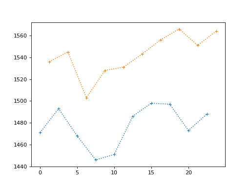
Now plot the first 10 values for the slice 0 times, against the first 10 values of the slice 0 time series.
Do the same plot for the first 10 values of the slice 1 times, against the first 10 values of the slice 1 time series.
Use the :+ line marker for the plots to get the actual position of the
points, and dotted lines between them.
>>> #- Plot first 10 values of slice 0 times against first 10 of slice 0
>>> #- time series;
>>> #- Plot first 10 values of slice 1 times against first 10 of slice 1
>>> #- time series.
>>> #- Use ':+' marker
>>> plt.plot(slice_0_times[:10], slice_0_ts[:10], ':+')
[...]
>>> plt.plot(slice_1_times[:10], slice_1_ts[:10], ':+')
[...]

Import InterpolatedUnivariateSpline from scipy.interpolate. Make a new
linear (k=1) interpolation object for slice 1, with the slice 1 times and
values.
>>> #- Import `InterpolatedUnivariateSpline` from `scipy.interpolate`
>>> #- Make a new linear (`k=1`) interpolation object for slice 1, with
>>> #- slice 1 times and values.
>>> from scipy.interpolate import InterpolatedUnivariateSpline
>>> interp = InterpolatedUnivariateSpline(slice_1_times, slice_1_ts, k=1)
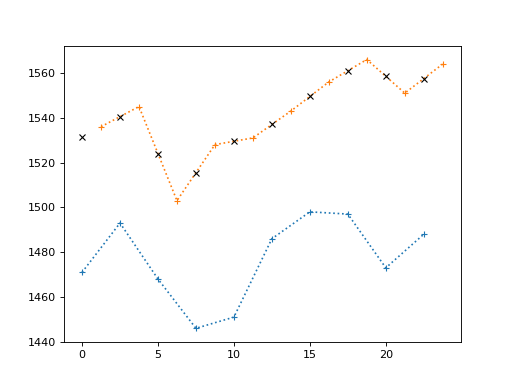
Call the object you got with the slice 0 times, to get the estimated time series values for slice 1, if slice 1 had been collected at the same time as slice 0:
>>> #- Call interpolator with `slice_0_times` to get estimated values
>>> slice_1_ts_est = interp(slice_0_times)
Repeat the plot of the first 10 values of the time series. This time, on the
same plot, add the estimated values for slice 1, if they had been collected at
the same time as slice 0. Use a black x for the estimated points (marker
'kx'):
>>> #- Plot first 10 values of slice 0 times against first 10 of slice 0
>>> #- time series;
>>> #- Plot first 10 values of slice 1 times against first 10 of slice 1
>>> #- time series;
>>> #- Plot first 10 values of slice 0 times against first 10 of
>>> #- interpolated slice 1 time series.
>>> plt.plot(slice_0_times[:10], slice_0_ts[:10], ':+')
[...]
>>> plt.plot(slice_1_times[:10], slice_1_ts[:10], ':+')
[...]
>>> plt.plot(slice_0_times[:10], slice_1_ts_est[:10], 'kx')
[...]

Use numpy to make a new copy of the data matrix. This will contain the slice time corrected values for all voxels. Copying the data matrix will give us the data we want for slice 0, because we want to keep the values for z slice 0 unchanged. We need to make a copy of the array to make sure we do not overwrite the original data.
>>> #- Copy old data to a new array
>>> new_data = fixed_data.copy()
Loop over every x voxel coordinate, and then loop over every y voxel coordinate.
For each x, y voxel coordinate:
- extract the time series at this x, y coordinate for slice 1;
- make a linear interpolator object with the slice 1 times and the extracted time series;
- resample this interpolator at the slice 0 times;
- put this new resampled time series into the new data at the same position.
>>> #- loop over all x coordinate values
>>> #- loop over all y coordinate values
>>> #- extract the time series at this x, y coordinate for slice 1;
>>> #- make a linear interpolator object with the slice 1 times and the
>>> #- extracted time series;
>>> #- resample this interpolator at the slice 0 times;
>>> #- put this new resampled time series into the new data at the same
>>> #- position.
>>> for x in range(fixed_data.shape[0]):
...     for y in range(fixed_data.shape[1]):
...         time_series = fixed_data[x, y, 1, :]
...         interp = InterpolatedUnivariateSpline(slice_1_times, time_series, k=1)
...         new_series = interp(slice_0_times)
...         new_data[x, y, 1, :] = new_series
Now we need to do the same thing for all the z slices.
To do this, we want to construct an offset vector (call it time_offset) of
length (number of z slices) such that adding the time_offset[z] to the
acquisition time of the first slice will give us the time of acquisition of
slice z. The next few steps are to get to that time_offset vector.
First, make a new vector acquisition_order that is length 30, where
acquisition_order[i] is the order of acquisition of slice index i. For
example, the first 4 elements of acqusition_order should be 0, 15, 1, 16.
>>> #- Make acquisition_order vector, length 30, with values:
>>> #- 0, 15, 1, 16 ... 14, 29
>>> acquisition_order = np.zeros(30)
>>> acquisition_index = 0
>>> for i in range(0, 30, 2):
...     acquisition_order[i] = acquisition_index
...     acquisition_index += 1
>>> for i in range(1, 30, 2):
...     acquisition_order[i] = acquisition_index
...     acquisition_index += 1
>>> acquisition_order
array([  0.,  15.,   1.,  16.,   2.,  17.,   3.,  18.,   4.,  19.,   5.,
        20.,   6.,  21.,   7.,  22.,   8.,  23.,   9.,  24.,  10.,  25.,
        11.,  26.,  12.,  27.,  13.,  28.,  14.,  29.])
Divide the acquisition order vector by number of slices, and multiply by the TR, to get the time offset for each z slice, relative to the start of the scan:
>>> #- Divide acquisition_order by number of slices, multiply by TR
>>> time_offsets = acquisition_order / 30 * TR
>>> time_offsets
array([ 0.    ,  1.25  ,  0.0833,  1.3333,  0.1667,  1.4167,  0.25  ,
        1.5   ,  0.3333,  1.5833,  0.4167,  1.6667,  0.5   ,  1.75  ,
        0.5833,  1.8333,  0.6667,  1.9167,  0.75  ,  2.    ,  0.8333,
        2.0833,  0.9167,  2.1667,  1.    ,  2.25  ,  1.0833,  2.3333,
        1.1667,  2.4167])
Now we can do our whole slice time correction, for every slice.
For each z coordinate (slice index):
Make a time vector by adding the slice time offset for this slice, to the
slice_0times. Call this theslice_z_timesvector;For each x coordinate:
For each y coordinate:
- extract the time series at this x, y, z coordinate;
- make a linear interpolator object with the
slice_z_timesand the extracted time series; - resample this interpolator at the slice 0 times;
- put this new resampled time series into the new data at the same position
>>> #- For each z coordinate (slice index):
>>> #- # Make `slice_z_times` vector for this slice
>>> #- ## For each x coordinate:
>>> #- ### For each y coordinate:
>>> #- #### extract the time series at this x, y, z coordinate;
>>> #- #### make a linear interpolator object with the `slice_z_times` and
>>> #-      the extracted time series;
>>> #- #### resample this interpolator at the slice 0 times;
>>> #- #### put this new resampled time series into the new data at the
>>> #-      same position
>>> for z in range(fixed_data.shape[2]):
...     slice_z_times = slice_0_times + time_offsets[z]
...     for x in range(fixed_data.shape[0]):
...         for y in range(fixed_data.shape[1]):
...             time_series = fixed_data[x, y, z, :]
...             interp = InterpolatedUnivariateSpline(slice_z_times, time_series, k=1)
...             new_series = interp(slice_0_times)
...             new_data[x, y, z, :] = new_series
Congratulations - you have just done slice timing correction on this 4D image.