\(\newcommand{L}[1]{\| #1 \|}\newcommand{VL}[1]{\L{ \vec{#1} }}\newcommand{R}[1]{\operatorname{Re}\,(#1)}\newcommand{I}[1]{\operatorname{Im}\, (#1)}\)
Smoothing exercise
>>> #: standard imports
>>> import numpy as np
>>> import matplotlib.pyplot as plt
>>> # print arrays to 4 decimal places
>>> np.set_printoptions(precision=4, suppress=True)
>>> import numpy.linalg as npl
>>> import nibabel as nib
>>> #: gray colormap and nearest neighbor interpolation by default
>>> plt.rcParams['image.cmap'] = 'gray'
>>> plt.rcParams['image.interpolation'] = 'nearest'
Smoothing and convolution
Start by smoothing in 1D. We first load a functional image
(ds114_sub009_t2r1.nii), and get the first volume:
>>> #: get first volume from functional
>>> import nibabel as nib
>>> img = nib.load('ds114_sub009_t2r1.nii')
>>> data = img.get_data()
>>> vol0 = data[..., 0]
Get a plane of the first volume by taking a slice on the third dimension:
>>> #: get slice over third dimension
>>> mid_slice = vol0[:, :, 14]
>>> plt.imshow(mid_slice)
<...>

Get one line of this slice, from left to right, from the middle of the brain:
>>> #: get middle line from middle slice
>>> mid_line = mid_slice[:, 25]
>>> plt.plot(mid_line)
[...]
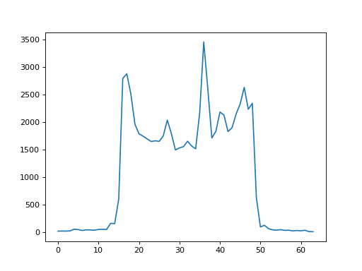
We are going to start by smoothing this line. This is smoothing in one dimension.
Here is the fwhm2sigma function from the page smoothing as convolution:
>>> #: Full-width at half-maximum to sigma
>>> def fwhm2sigma(fwhm):
...     return fwhm / np.sqrt(8 * np.log(2))
Here is a test that the function returns an expected result:
>>> #: Test output of fwhm2sigma for a single FWHM
>>> assert np.allclose(fwhm2sigma(4), 1.698643600576)
We are going to smooth by 8 pixels full-width at half maximum (FWHM), so we
need the corresponding sigma (standard deviation):
>>> #- sigma for FWHM 8?
>>> sigma = fwhm2sigma(8)
>>> sigma
3.3972872011520763
We use the probability density function (PDF) of a Gaussian distribution for our kernel:
where:
To make our smoothing kernel, we can sample the PDF, for a given \(\mu\) and \(\sigma\).
We can use scipy.stats to sample from the PDF.
>>> #: import the Gaussian (normal) distribution function
>>> from scipy.stats import norm
>>> norm_pdf = norm.pdf
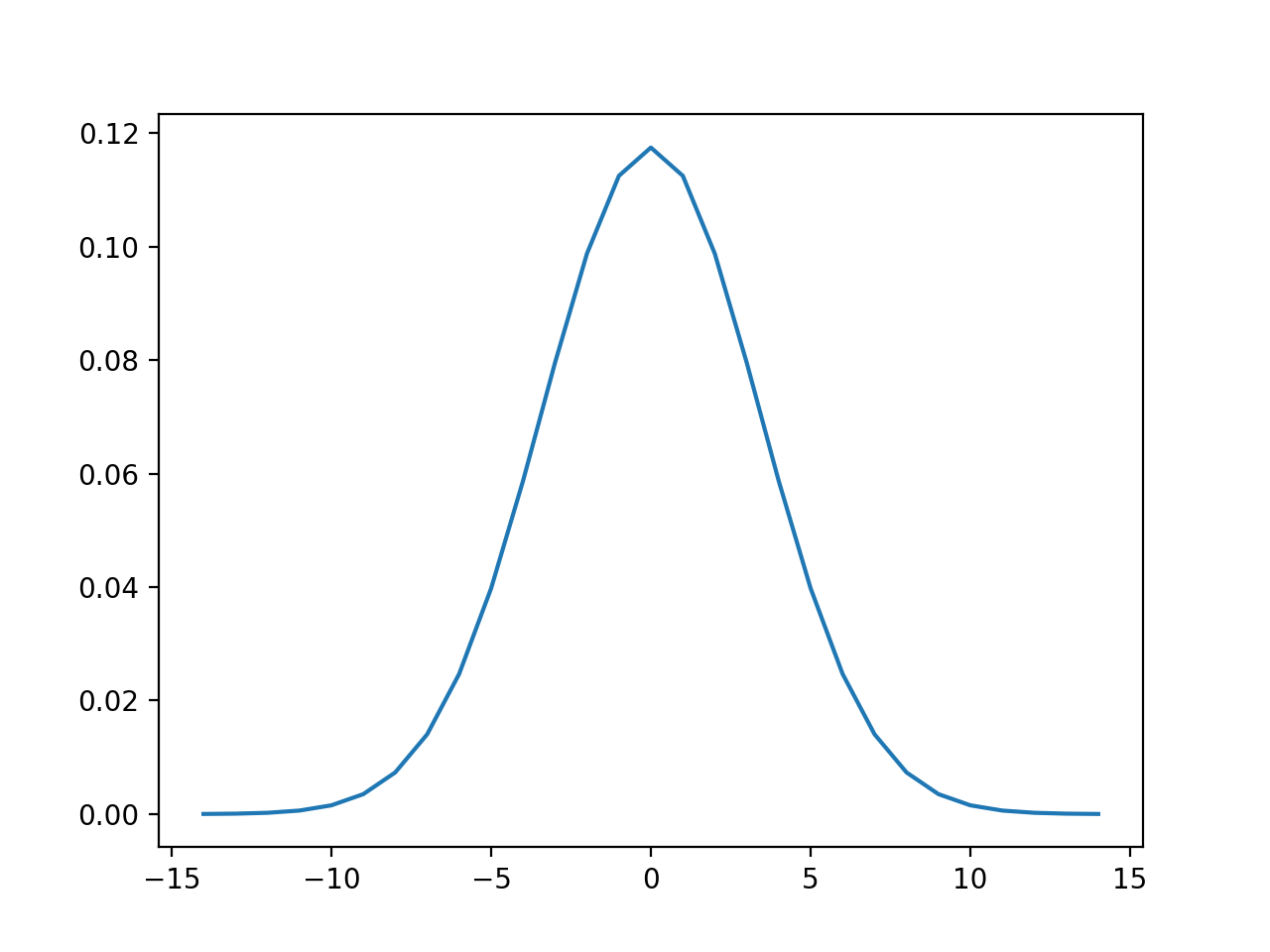
Next we need to make our smoothing kernel from values in the Gaussian PDF:
- Work out the +/- limit for the kernel x values with
limit = round(sigma * 4) - Make a vector of integers
xto sample the PDF from-limittolimit- inclusive; - Sample the PDF at these x values, for \(\mu = 0\) and given
\(\sigma\), to get the
kernelvector; - Plot the x values against the y values;
- Work out how many elements there are from the start of the
kernelvector, to the value corresponding to \(x=0\) – this is thekernel_offset.
>>> #- Work out the +/- limit for the kernel x values;
>>> #- Make a vector `x` to sample the PDF;
>>> #- Get `kernel` vector by sampling the PDF at these x values (mu=0);
>>> #- Work out `kernel_offset`.
>>>
>>> limit = round(sigma * 4)
>>> # Make an x range between -sigma * 3 and +sigma * 3
>>> x_for_kernel = np.arange(-limit, limit+1)
>>> # Calculate kernel
>>> kernel = norm_pdf(x_for_kernel, 0, sigma)
>>> # Plot kernel
>>> plt.plot(x_for_kernel, kernel)
[...]
>>> # Calculate `kernel_offset`
>>> kernel_offset = int(limit)
>>> kernel_offset
14
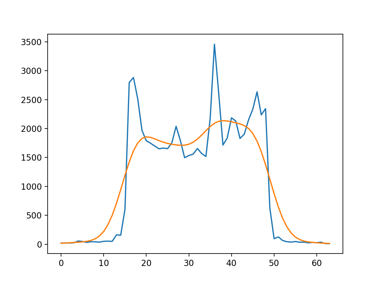
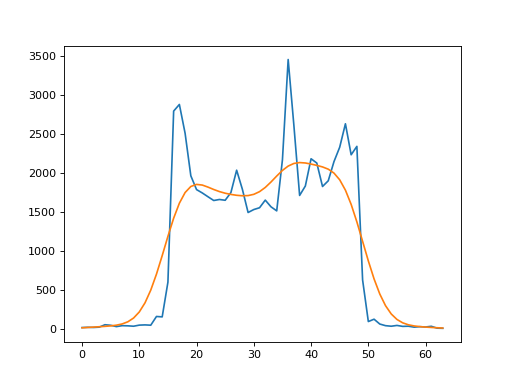
Now we can convolve the line from the image plane with the kernel. We take
the result starting at kernel_offset:
>>> #- Convolve image line with kernel
>>> #- Slice out the result we want using kernel_offset
>>> #- Plot smoothed with unsmoothed line
>>> smoothed = np.convolve(mid_line, kernel)
>>> smoothed = smoothed[kernel_offset:len(mid_line)+kernel_offset]
>>> plt.plot(mid_line)
[...]
>>> plt.plot(smoothed)
[...]
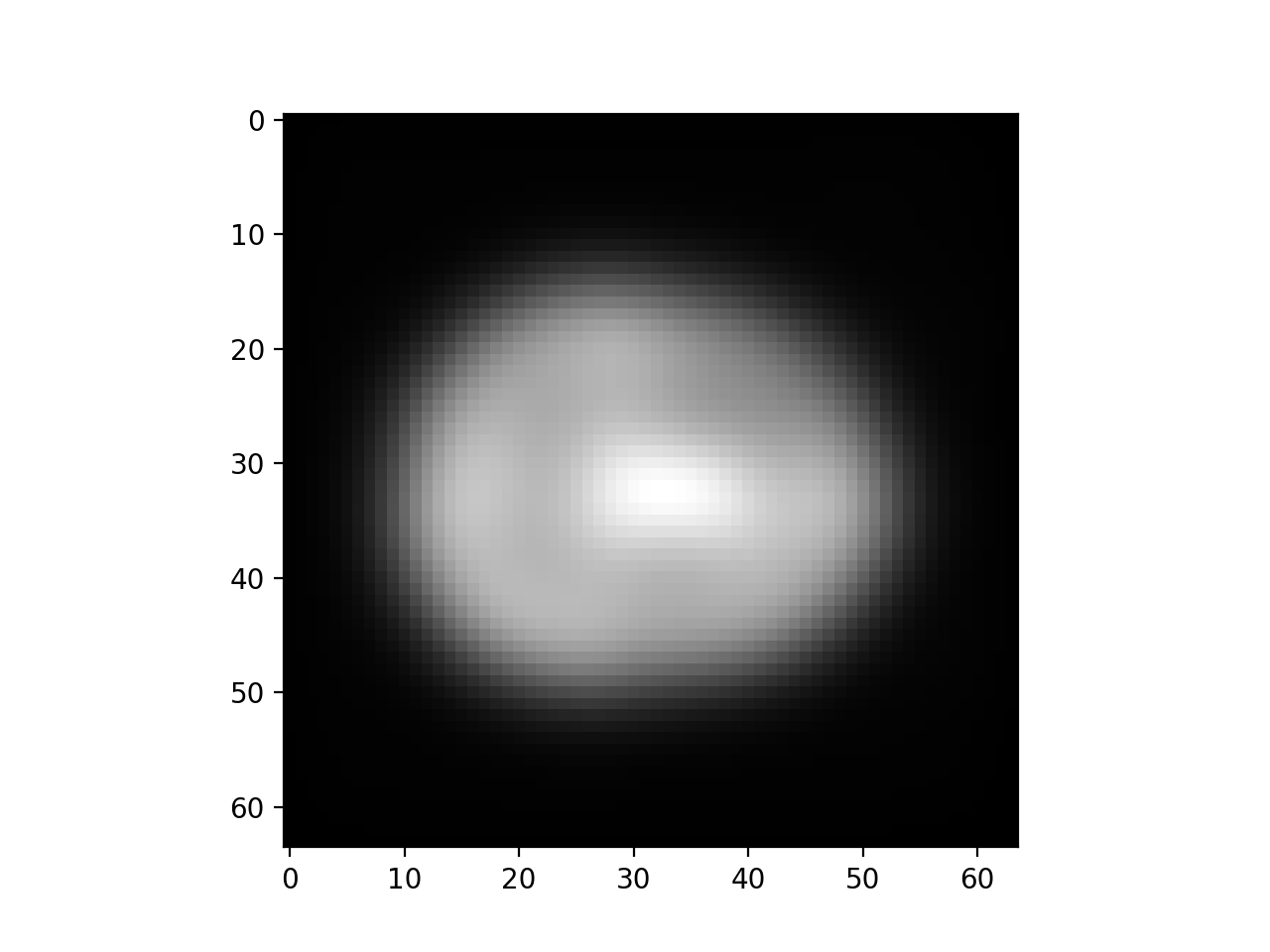
Smoothing the whole image slice is a simple extension. It turns out that we can apply smoothing in two dimensions, by first applying the smoothing to each line in one dimension. Then we take the output of this smoothing and apply the smoothing to the second dimension.
- Make a new array the same shape as
mid_slicecalledsmoothed_slice; - Loop over the first dimension of
mid_slice, and fill each line ofsmoothed_slicewith the smoothed version; - Loop over the second dimension of
smoothed_sliceand replace each line with the smoothed version; - Show.
>>> #- Make a new array `smoothed_slice` for smoothed output
>>> #- Loop over first dimension applying kernel as above
>>> #- Loop over second dimension of smoothed image, applying kernel
>>> #- Show with `imshow`
>>> smoothed_slice = np.zeros(mid_slice.shape)
>>> n_x, n_y = mid_slice.shape
>>> for x in range(n_x):
...     line = mid_slice[x, :]
...     smoothed = np.convolve(line, kernel)
...     smoothed_slice[x, :] = smoothed[kernel_offset:n_y+kernel_offset]
>>> for y in range(n_y):
...     line = smoothed_slice[:, y]
...     smoothed = np.convolve(line, kernel)
...     smoothed_slice[:, y] = smoothed[kernel_offset:n_x+kernel_offset]
>>> plt.imshow(smoothed_slice)
<...>

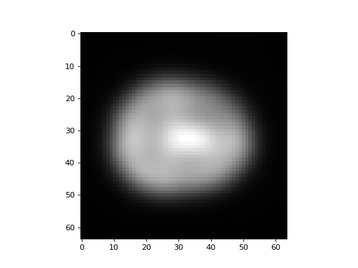
We can do the same thing with scipy.ndimage.gaussian_filter.
>>> #: import gaussian_filter
>>> from scipy.ndimage import gaussian_filter
Have a look at the help for gaussian_filter.
Use gaussian_filter to make another smoothed version of mid_slice.
>>> #- Use gaussian filter to smooth `mid_slice`
>>> scipy_slice = gaussian_filter(mid_slice, sigma)
>>> plt.imshow(scipy_slice)
<...>

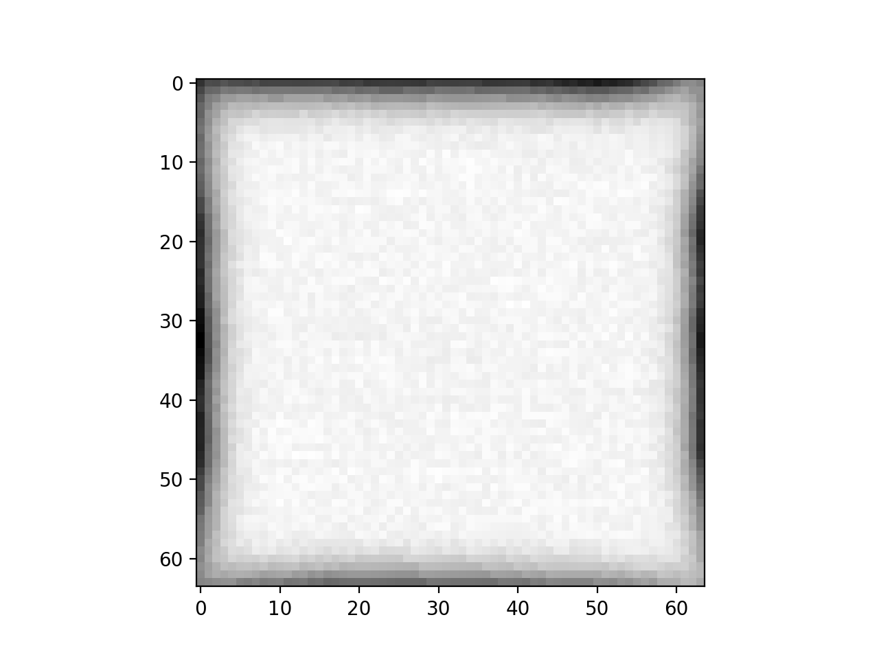
Subtract the gaussian_filter version from your handcrafted version.
Can you explain the difference?
>>> #- Subtract two versions of the smoothed slice, show
>>> diff_slice = smoothed_slice - scipy_slice
>>> plt.imshow(diff_slice)
<...>
