\(\newcommand{L}[1]{\| #1 \|}\newcommand{VL}[1]{\L{ \vec{#1} }}\newcommand{R}[1]{\operatorname{Re}\,(#1)}\newcommand{I}[1]{\operatorname{Im}\, (#1)}\)
Predicted neural time course exercise
- For code template see:
hrf_correlation_code.py; - For solution see: Predicted neural time course exercise.
>>> #: Standard imports
>>> import numpy as np
>>> import matplotlib.pyplot as plt
>>> # Print arrays to 4 decimal places
>>> np.set_printoptions(precision=4, suppress=True)
We are going to be analyzing the data for the 4D image
ds114_sub009_t2r1.nii again.
Load the image into an image object with nibabel, and get the image data array. Print the shape.
>>> #- Load the image with nibabel.
>>> #- Get the image data array, print the data shape.
Next we read in the stimulus file for this run to make an on - off time-series.
The stimulus file is ds114_sub009_t2r1_cond.txt.
Here’s a version of the same thing we did in First go at brain activation exercise, wrapped up as a function:
>>> #: Read in stimulus file, return neural prediction
>>> def events2neural(task_fname, tr, n_trs):
...     """ Return predicted neural time course from event file
...
...     Parameters
...     ----------
...     task_fname : str
...         Filename of event file
...     tr : float
...         TR in seconds
...     n_trs : int
...         Number of TRs in functional run
...
...     Returns
...     -------
...     time_course : array shape (n_trs,)
...         Predicted neural time course, one value per TR
...     """
...     task = np.loadtxt(task_fname)
...     if task.ndim != 2 or task.shape[1] != 3:
...         raise ValueError("Is {0} really a task file?", task_fname)
...     task[:, :2] = task[:, :2] / tr
...     time_course = np.zeros(n_trs)
...     for onset, duration, amplitude in task:
...         onset, duration = int(onset),  int(duration)
...         time_course[onset:onset + duration] = amplitude
...     return time_course
Use this function to read ds114_sub009_t2r1_cond.txt and return a
predicted neural time course.
The TR for this run is 2.5. You know the number of TRs from the image data shape above.
>>> #: TR for this run
>>> tr = 2.5
>>> #- Read the stimulus data file and return a predicted neural time
>>> #- course.
>>> #- Plot the predicted neural time course.
We had previously found that the first volume in this run was bad. Use your
slicing skills to make a new array called data_no_0 that is the data array
without the first volume:
>>> #- Make new array excluding the first volume
>>> #- data_no_0 = ?
Our neural prediction time series currently has one value per volume,
including the first volume. To match the data, make a new neural prediction
variable that does not include the first value of the time series. Call this
new variable neural_prediction_no_0.
>>> #- Knock the first element off the neural prediction time series.
>>> #- neural_prediction_no_0 = ?
For now, we’re going to play with data for a single voxel.
In First go at brain activation exercise, we subtracted the rest scans from the task scans, something like this:
>>> #: subtracting rest from task scans
>>> task_scans = data_no_0[..., neural_prediction_no_0 == 1]
>>> rest_scans = data_no_0[..., neural_prediction_no_0 == 0]
>>> difference = task_scans.mean(axis=-1) - rest_scans.mean(axis=-1)
>>> #: showing slice 14 from the difference image
>>> plt.imshow(difference[:, :, 14], cmap='gray')
<...>
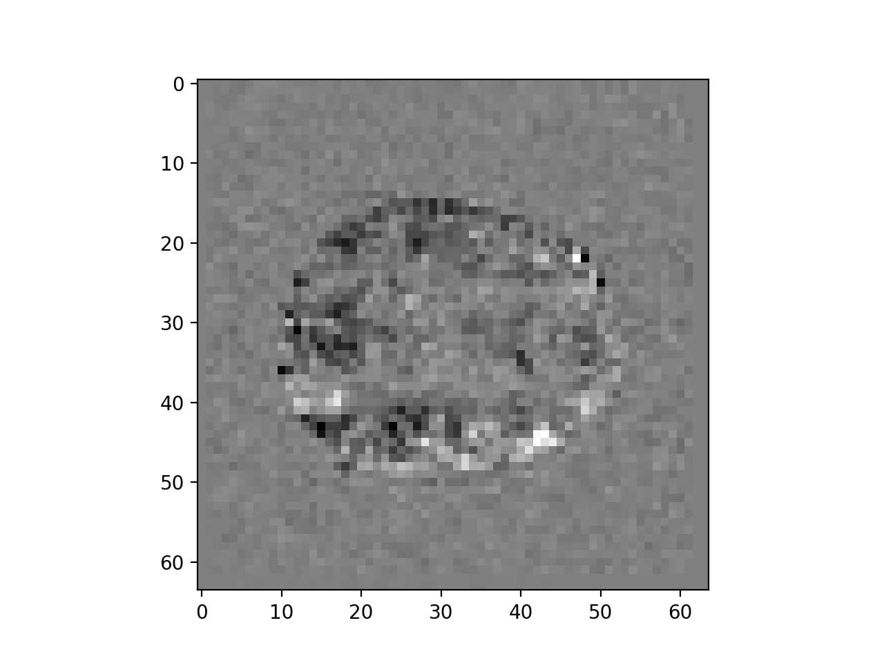
It looks like there’s a voxel that is greater for activation than rest at about (i, j, k) == (45, 43, 14).
Get and plot the values for this voxel position, for every volume in the 4D data (not including the first volume). You can do it with a loop, but slicing is much nicer.
>>> #- Get the values for (i, j, k) = (45, 43, 14) and every volume.
>>> #- Plot the values (voxel time course).
Correlate the predicted neural time series with the voxel time course:
>>> #- Correlation of predicted neural time course with voxel signal time
>>> #- course
Now we will do a predicted hemodynamic time course using convolution.
Next we need to get the HRF vector to convolve with.
Here is my not-that-good HRF definition. Feel free to replace this one with your better HRF definition from Making our own hemodynamic response function:
>>> #: import the gamma probability density function
>>> from scipy.stats import gamma
>>>
>>> def mt_hrf(times):
...     """ Return values for HRF at given times
...
...     This is the "not_great_hrf" from the "make_an_hrf" exercise.
...     Feel free to replace this function with your improved version from
...     that exercise.
...     """
...     # Gamma pdf for the peak
...     peak_values = gamma.pdf(times, 6)
...     # Gamma pdf for the undershoot
...     undershoot_values = gamma.pdf(times, 12)
...     # Combine them
...     values = peak_values - 0.35 * undershoot_values
...     # Scale max to 0.6
...     return values / np.max(values) * 0.6
Remember we have defined the HRF as a function of time, not TRs.
For our convolution, we need to sample the HRF at times corresponding the start of the TRs.
So, we need to sample at times (0, 2.5, …)
Make a vector of times at which to sample the HRF. We want to sample every TR up until (but not including) somewhere near 35 seconds (where the HRF should have got close to zero again).
>>> #- Make a vector of times at which to sample the HRF
Sample your HRF function at these times and plot:
>>> #- Sample HRF at given times
>>> #- Plot HRF samples against times
Convolve the predicted neural time course with the HRF samples:
>>> #- Convolve predicted neural time course with HRF samples
The default output of convolve is longer than the input neural prediction vector, by the length of the convolving vector (the HRF samples) minus 1. Knock these last values off the result of the convolution to get a vector the same length as the neural prediction:
>>> #- Remove extra tail of values put there by the convolution
Plot the convolved neural prediction, and then, on the same plot, plot the unconvolved neural prediction.
>>> #- Plot convolved neural prediction and unconvolved neural prediction
Does the new convolved time course correlate better with the voxel time course?
>>> #- Correlation of the convolved time course with voxel time course
Plot the hemodynamic prediction against the actual signal (voxel values). Remember to use a marker such as ‘+’ to give you a scatter plot. How does it look?
>>> #- Scatterplot the hemodynamic prediction against the signal