\(\newcommand{L}[1]{\| #1 \|}\newcommand{VL}[1]{\L{ \vec{#1} }}\newcommand{R}[1]{\operatorname{Re}\,(#1)}\newcommand{I}[1]{\operatorname{Im}\, (#1)}\)

Otsu’s method for binarizing images

This page has some notes explaining Otsu’s method for binarizing grayscale images.

The best source on the method is the original paper. At the time I wrote this page, the Wikipedia article is too messy to be useful.

Conceptually, Otsu’s method proceeds like this:

• create the 1D histogram of image values, where the histogram has \(L\) bins. The histogram is \(L\) bin counts \(\vec{c} = [c_1, c_2, ... c_L]\), where \(c_i\) is the number of values falling in bin \(i\). The histogram has bin centers \(\vec{v} = [v_1, v_2, ..., v_L]\), where \(v_i\) is the image value corresponding to the center of bin \(i\);

• for every bin number \(k \in [1, 2, 3, ..., L-1]\), divide the histogram at that bin to form a left histogram and a right histogram, where the left histogram has counts, centers \([c_1, ... c_k], [v_1, ... v_k]\), and the right histogram has counts, centers \([c_{k+1} ... c_L], [v_{k+1} .. v_L]\);

• calculate the mean corresponding to the values in the left and right histogram:

  \[\begin{split}n_k^{left} = \sum_{i=1}^{k} c_i \\ \mu_k^{left} = \frac{1}{n_k^{left}} \sum_{i=1}^{k} c_i v_i \\ n_k^{right} = \sum_{i={k+1}}^{L} c_i \\ \mu_k^{right} = \frac{1}{n_k^{right}} \sum_{i={k+1}}^{L} c_i v_i\end{split}\]

• calculate the sum of squared deviations from the left and right means:

  \[\begin{split}\mathrm{SSD}_k^{left} = \sum_{i=1}^{k} c_i (v_i - \mu_k^{left}) \\ \mathrm{SSD}_k^{right} = \sum_{i={k+1}}^{L} c_i (v_i - \mu_k^{right}) \\ \mathrm{SSD}_k^{total} = SSD_k^{left} + SSD_k^{right}\end{split}\]

• find the bin number \(k\) that minimizes \(\mathrm{SSD}_k^{total}\):

  \[z = \mathrm{argmin}_k \mathrm{SSD}_k^{total}\]

• the binarizing threshold for the image is the value corresponding to this bin \(z\):

  \[t = v_z\]

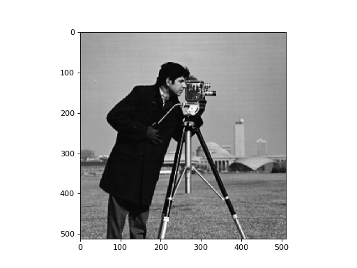
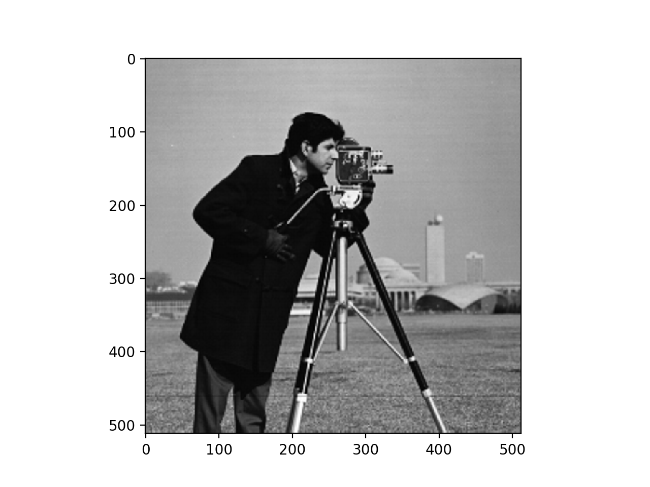
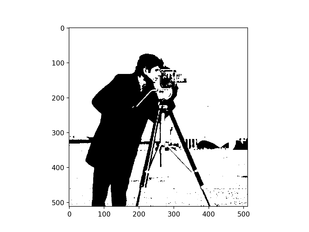
Here is Otsu’s threshold in action. First we load an image:

>>> import numpy as np
>>> import matplotlib.pyplot as plt
>>> cameraman = np.loadtxt('camera.txt').reshape((512, 512))
>>> plt.imshow(cameraman.T, cmap='gray', interpolation='nearest')
<...>

(png, hires.png, pdf)

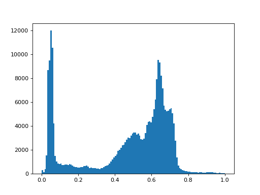
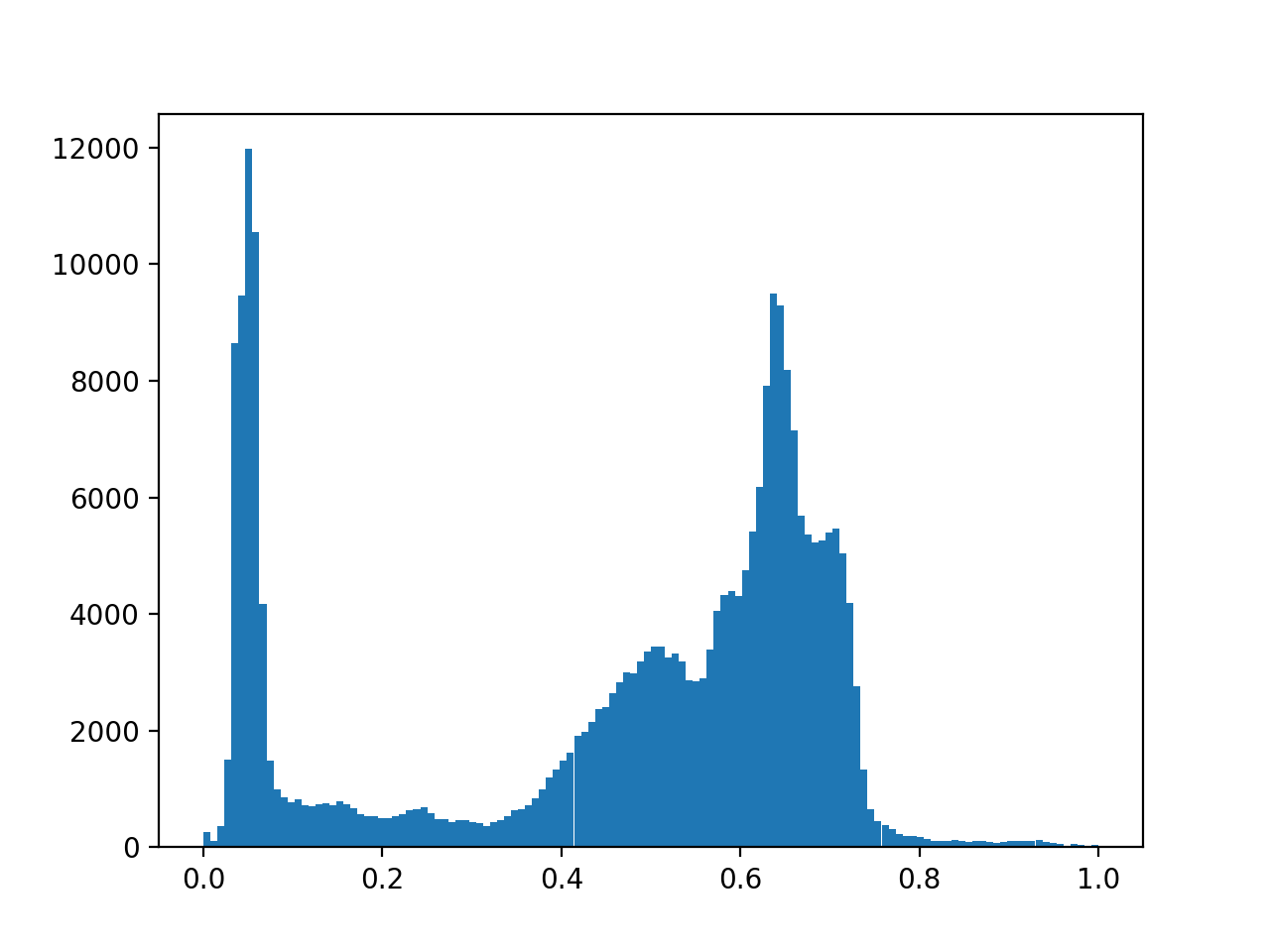
Make a histogram:

>>> cameraman_1d = cameraman.ravel()
>>> n_bins = 128
>>> plt.hist(cameraman_1d, bins=n_bins)
(...)
>>> counts, edges = np.histogram(cameraman, bins=n_bins)
>>> bin_centers = edges[:-1] + np.diff(edges) / 2.

(png, hires.png, pdf)

Calculate the threshold:

>>> def ssd(counts, centers):
...     """ Sum of squared deviations from mean """
...     n = np.sum(counts)
...     mu = np.sum(centers * counts) / n
...     return np.sum(counts * ((centers - mu) ** 2))

>>> total_ssds = []
>>> for bin_no in range(1, n_bins):
...     left_ssd = ssd(counts[:bin_no], bin_centers[:bin_no])
...     right_ssd = ssd(counts[bin_no:], bin_centers[bin_no:])
...     total_ssds.append(left_ssd + right_ssd)
>>> z = np.argmin(total_ssds)
>>> t = bin_centers[z]
>>> print('Otsu bin (z):', z)
Otsu bin (z): 43
>>> print('Otsu threshold (c[z]):', bin_centers[z])
Otsu threshold (c[z]): 0.33984375

This gives the same result as the scikit-image implementation:

>>> from skimage.filters import threshold_otsu
>>> threshold_otsu(cameraman, n_bins)
0.33984375
>>> np.allclose(threshold_otsu(cameraman, n_bins), t)
True

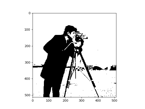
The original image binarized with this threshold:

>>> binarized = cameraman > t
>>> plt.imshow(binarized.T, cmap='gray', interpolation='nearest')
<...>

(png, hires.png, pdf)