\(\newcommand{L}[1]{\| #1 \|}\newcommand{VL}[1]{\L{ \vec{#1} }}\newcommand{R}[1]{\operatorname{Re}\,(#1)}\newcommand{I}[1]{\operatorname{Im}\, (#1)}\)

Whole-brain t tests and p values

Here we do a whole brain analysis on our example dataset:

>>> import numpy as np
>>> np.set_printoptions(precision=4)  # print arrays to 4 dp
>>> import numpy.linalg as npl
>>> import matplotlib.pyplot as plt
>>> import nibabel as nib

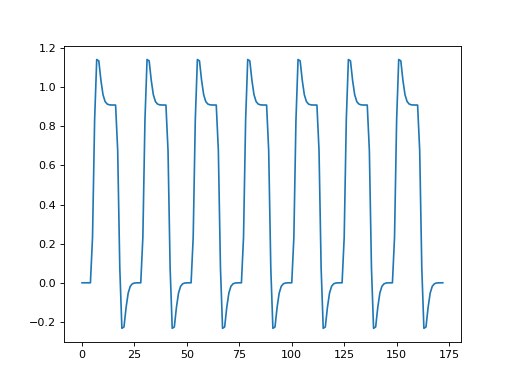
We load the hemodynamic regressor from Convolving with the hemodyamic response function. We used this regressor in Modeling a single voxel:

>>> regressor = np.loadtxt('ds114_sub009_t2r1_conv.txt')
>>> plt.plot(regressor)
[...]

(png, hires.png, pdf)

Load the FMRI data, drop the first four volumes:

>>> data = nib.load('ds114_sub009_t2r1.nii').get_data()
>>> data = data[..., 4:]
>>> data.shape
(64, 64, 30, 169)
>>> n = data.shape[-1]

Drop the matching time points in the regressor:

>>> regressor = regressor[4:]

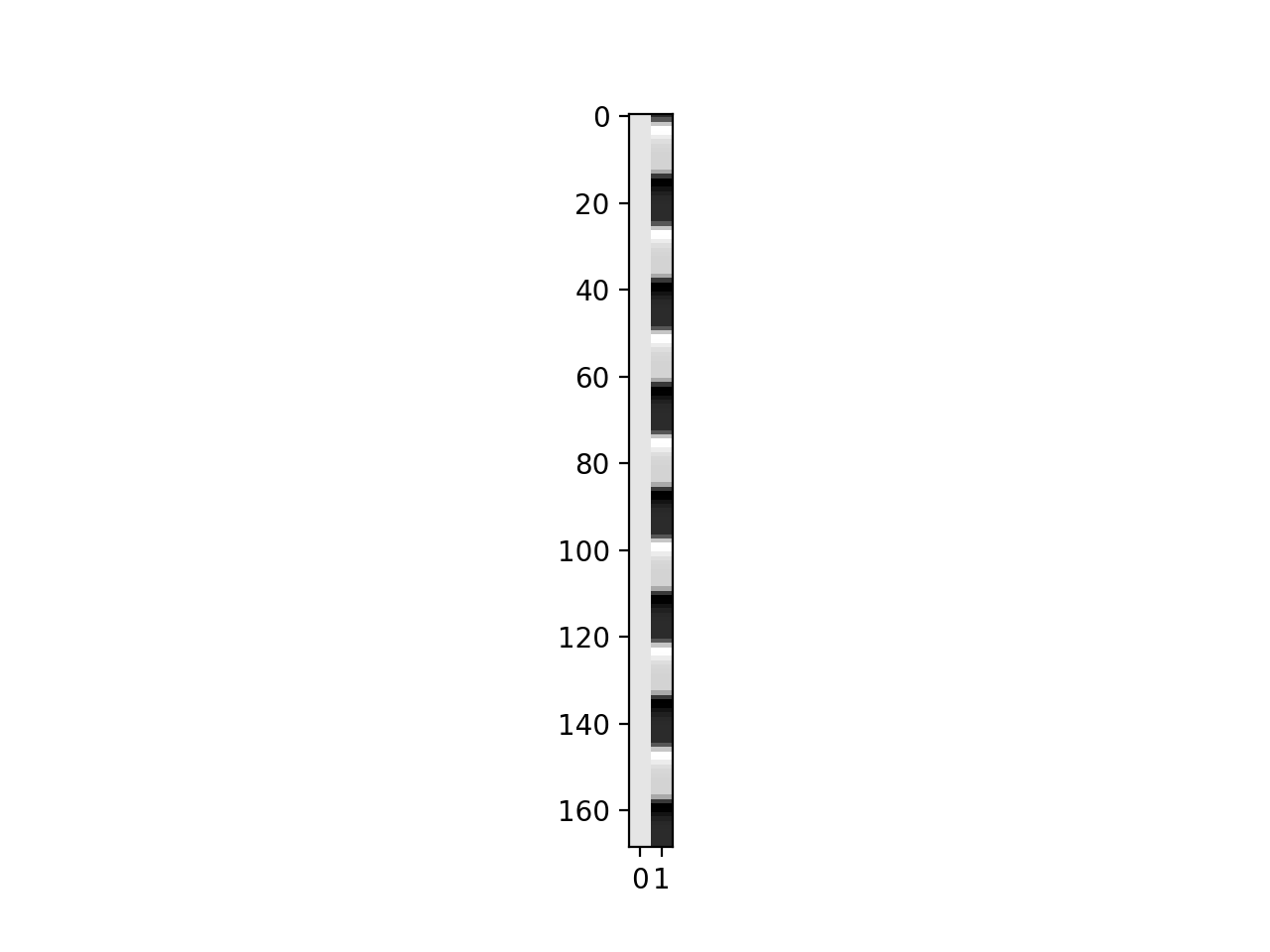
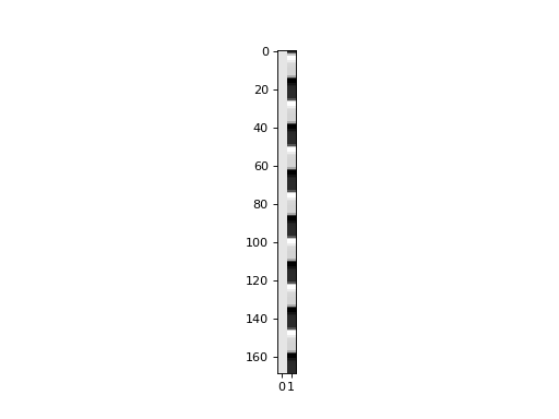
Make the design matrix for the simple regression:

>>> X = np.ones((n, 2))
>>> X[:, 1] = regressor
>>> plt.imshow(X, cmap='gray', aspect=0.2)
<...>

(png, hires.png, pdf)

Analysis on whole volume, reshaped

Reshape data to time by voxels:

>>> Y = data.reshape((-1, n))
>>> Y = Y.T
>>> Y.shape
(169, 122880)

Fit the design to the data:

\[ \begin{align}\begin{aligned}\newcommand{\yvec}{\vec{y}} \newcommand{\xvec}{\vec{x}} \newcommand{\evec}{\vec{\varepsilon}} \newcommand{Xmat}{\boldsymbol X} \newcommand{\bvec}{\vec{\beta}} \newcommand{\bhat}{\hat{\bvec}} \newcommand{\yhat}{\hat{\yvec}} \newcommand{\ehat}{\hat{\evec}} \newcommand{\cvec}{\vec{c}} \newcommand{\rank}{\textrm{rank}}\\\yvec = \Xmat \bvec + \evec\end{aligned}\end{align} \]

Here we calculate the fit for all the columns in Y in one shot - see Estimation for many voxels at the same time:

>>> B = npl.pinv(X).dot(Y)
>>> B.shape
(2, 122880)

Contrast to test the difference of the slope from 0:

>>> c = np.array([0, 1])

Numerator of t test:

\[ \begin{align}\begin{aligned}\begin{split}\newcommand{\cvec}{\vec{c}} \hat\sigma^2 = \frac{1}{n - \rank(\Xmat)} \sum e_i^2 \\\end{split}\\t = \frac{\cvec^T \bhat} {\sqrt{\hat{\sigma}^2 \cvec^T (\Xmat^T \Xmat)^+ \cvec}}\end{aligned}\end{align} \]

>>> top_of_t = c.dot(B)
>>> top_of_t.shape
(122880,)

This selected the second row of the B array:

>>> np.all(top_of_t == B[1, :])
True

The denominator of the t statistic:

>>> df_error = n - npl.matrix_rank(X)
>>> df_error
167
>>> n
169
>>> fitted = X.dot(B)
>>> E = Y - fitted
>>> E.shape
(169, 122880)
>>> sigma_2 = np.sum(E ** 2, axis=0) / df_error
>>> c_b_cov = c.dot(npl.pinv(X.T.dot(X))).dot(c)
>>> c_b_cov
0.0238...

Here we left c as a 1D vector, and let the default of the dot method treat the 1D vector as a row vector on the left, and as a column vector on the right. See: Dot, vectors and matrices.

>>> c
array([0, 1])
>>> c.shape
(2,)

We could also make c into an explicit row vector to match the formula of the t statistic above. See Adding length 1 dimensions with newaxis:

>>> c = c[:, None]
>>> c.shape
(2, 1)
>>> c_b_cov = c.T.dot(npl.pinv(X.T.dot(X))).dot(c)
>>> c_b_cov
array([[ 0.0238]])

Now we can have the parts that we need for the denominator, we can calculate the t statistic, one for each voxel:

>>> t = top_of_t / np.sqrt(sigma_2 * c_b_cov)
>>> t.shape
(1, 122880)

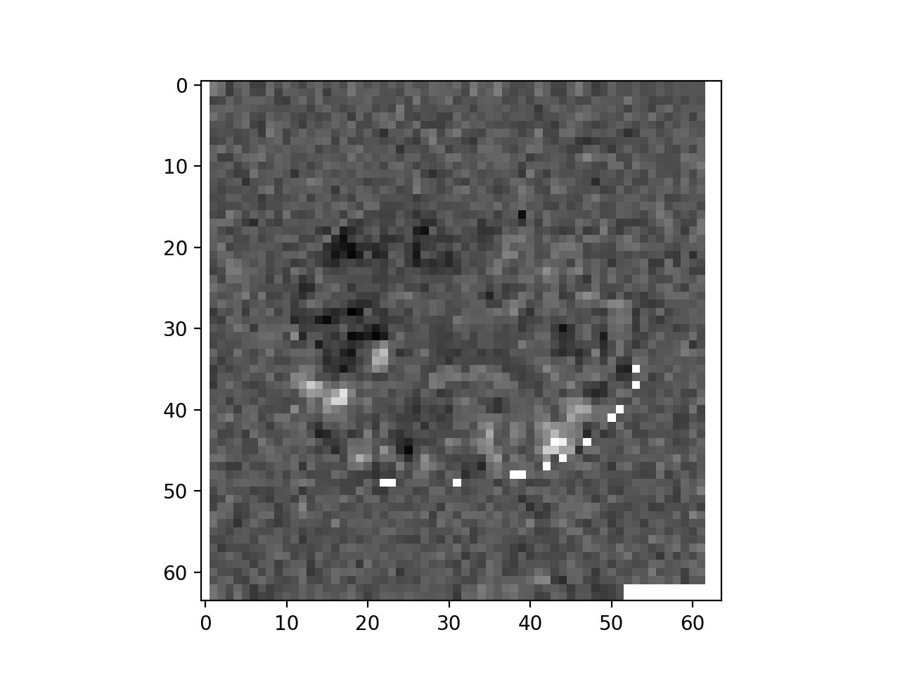
Reshape the 1D t statistic vector back into three dimensions to put the t statistic back into the correct voxel position:

>>> t_3d = t.reshape(data.shape[:3])
>>> t_3d.shape
(64, 64, 30)
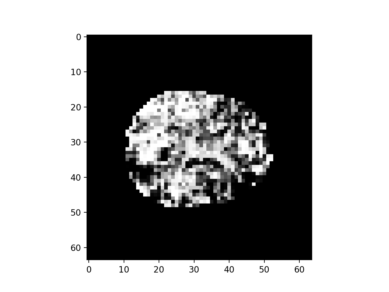
>>> plt.imshow(t_3d[:, :, 15], cmap='gray')
<...>

(png, hires.png, pdf)

Notice the white areas at the edge of the image. These are voxels where the t value is nan – Not a number. See also Not a number. nan values arise when all the scans have 0 at this voxel, so the numerator and denominator of the t statistic are both 0.

>>> np.array(0) / 0
nan

For example, this is the voxel corresponding to the top left corner of the image above:

>>> t_3d[0, 0, 15]
nan
>>> np.all(data[0, 0, 15] == 0)  #doctest: +SKIP
True
>>> sigma_2_3d = sigma_2.reshape(data.shape[:3])
>>> sigma_2_3d[0, 0, 15]
0.0

Can we avoid these uninteresting voxels, and only analyze voxels within the brain?

Analysis on voxels within the brain

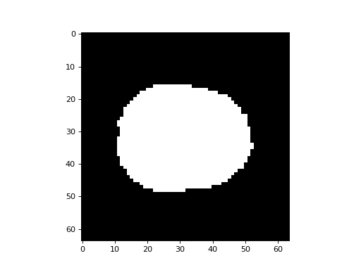
Here we make a mask of the voxels within the brain using Otsu’s method. You will need scikit-image installed for this to work:

>>> from skimage.filters import threshold_otsu
>>> mean = data.mean(axis=-1)
>>> mean.shape
(64, 64, 30)
>>> thresh = threshold_otsu(mean)
>>> thresh
849.70914...
>>> # The mask has True for voxels above "thresh", False otherwise
>>> mask = mean > thresh
>>> mask.shape
(64, 64, 30)
>>> plt.imshow(mask[:, :, 15], cmap='gray')
<...>
>>> data.shape
(64, 64, 30, 169)

(png, hires.png, pdf)

This is the number of voxels for which the mask value is True:

>>> np.sum(mask)  # doctest: +SKIP
21604

We can use the 3D mask to slice into the 4D data matrix. For every True value in the 3D mask, the result has the vector of values over time for that voxel. See: Indexing with boolean masks.

>>> Y = data[mask]
>>> Y.shape
(21604, 169)

For our GLM, we want a time by in-mask voxel array, which is the transpose of the result above:

>>> Y = data[mask].T
>>> Y.shape
(169, 21604)

Now we can run our GLM on the voxels inside the brain:

>>> B = npl.pinv(X).dot(Y)
>>> fitted = X.dot(B)
>>> E = Y - fitted
>>> sigma_2 = np.sum(E ** 2, axis=0) / df_error
>>> # c and c_b_cov are the same as before, but recalculate anyway
>>> c = np.array([0, 1])
>>> c_b_cov = c.dot(npl.pinv(X.T.dot(X))).dot(c)
>>> t = c.T.dot(B) / np.sqrt(sigma_2 * c_b_cov)
>>> t.shape
(21604,)

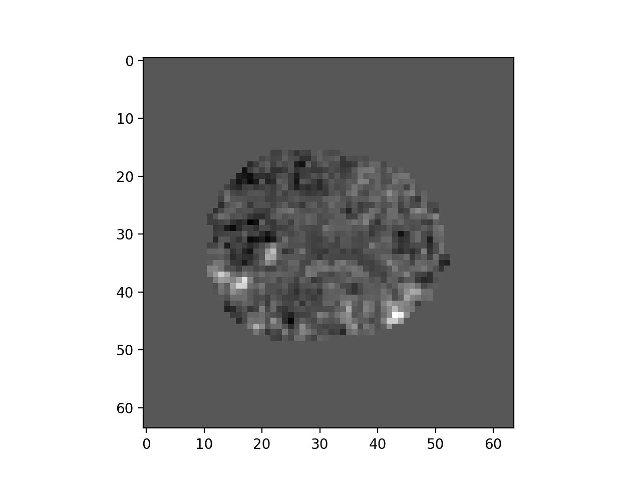
We can put the t values back into their correct positions in 3D by using the mask as an index on the left hand side:

>>> t_3d = np.zeros(data.shape[:3])
>>> t_3d[mask] = t
>>> plt.imshow(t_3d[:, :, 15], cmap='gray')
<...>

(png, hires.png, pdf)

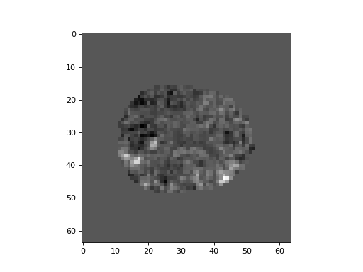
Now we calculate the p value for each t statistic:

>>> import scipy.stats as stats
>>> t_dist = stats.t(df_error)
>>> p = 1 - t_dist.cdf(t)
>>> p.shape
(21604,)
>>> p_3d = np.zeros(data.shape[:3])
>>> p_3d[mask] = p
>>> plt.imshow(p_3d[:, :, 15], cmap='gray')
<...>

(png, hires.png, pdf)

Multiple comparison correction

We now have a very large number of t statistics and p values. We want to find to control the family-wise error rate, where the “family” is the set of all of the voxel t tests / p values. See: Bonferroni correction.

We start with the Šidák correction, that gives the correct threshold when all the test are independent:

>>> N = p.shape[0]
>>> sidak_thresh = 1 - (1 - 0.05) ** (1./N)
>>> sidak_thresh
2.3742...e-06

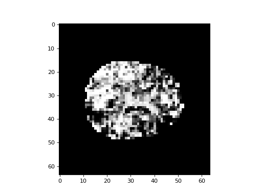
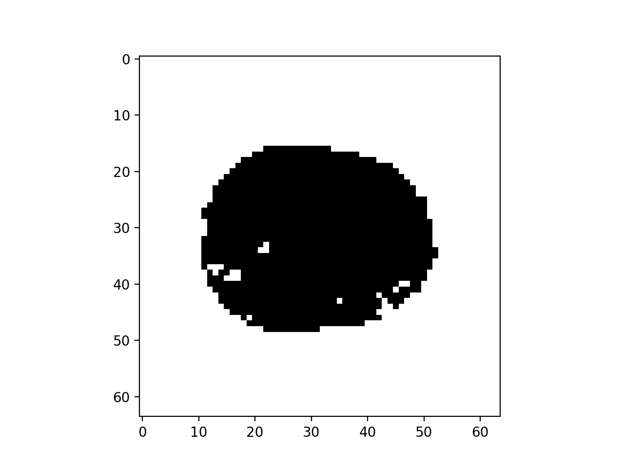
Binarize the voxel p values at the Šidák correction threshold, so voxels surviving correction have True, other voxels have False:

>>> plt.imshow(p_3d[:, :, 15] < sidak_thresh, cmap='gray')
<...>

(png, hires.png, pdf)

The voxels outside the brain have p value 0 (see above), so these always survive the correction above, and appear white.

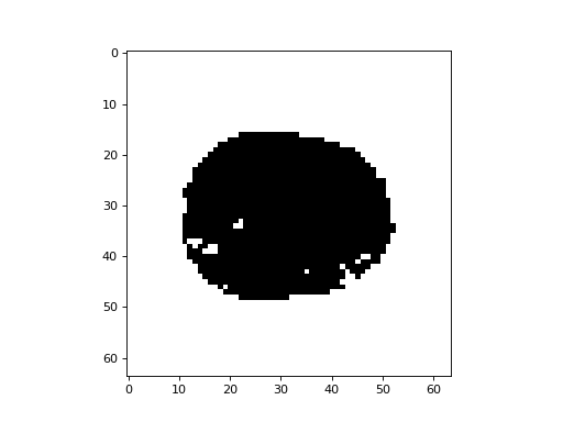
Now we threshold at the Bonferroni correction level. This does not assume the tests are independent:

>>> bonferroni_theta = 0.05 / N
>>> bonferroni_theta
2.3143...e-06
>>> plt.imshow(p_3d[:, :, 15] < bonferroni_theta, cmap='gray')
<...>

(png, hires.png, pdf)