\(\newcommand{L}[1]{\| #1 \|}\newcommand{VL}[1]{\L{ \vec{#1} }}\newcommand{R}[1]{\operatorname{Re}\,(#1)}\newcommand{I}[1]{\operatorname{Im}\, (#1)}\)
Affine optimization exercise
- For code template see:
optimizing_affine_code.py; - For solution see: Affine optimization exercise.
>>> #: standard imports
>>> import numpy as np
>>> import matplotlib.pyplot as plt
>>> # print arrays to 4 decimal places
>>> np.set_printoptions(precision=4, suppress=True)
>>> import numpy.linalg as npl
>>> import nibabel as nib
>>> #: gray colormap and nearest neighbor interpolation by default
>>> plt.rcParams['image.cmap'] = 'gray'
>>> plt.rcParams['image.interpolation'] = 'nearest'
We need the rotations.py code:
>>> #: Check import of rotations code
>>> from rotations import x_rotmat, y_rotmat, z_rotmat
An affine normalization
In Optimizing rotation exercise we used optimization to find what rotations I had applied to a functional volume.
Now we’re going to have a shot at using optimization to do an affine spatial normalization.
First – the images. We will be using skull-stripped version of the
structural image we have been using for the other exercises –
ds114_sub009_highres_brain_222.nii.
The skull-stripped version comes from the OpenFMRI dataset, but the authors
have used the FSL bet utility to do the skull stripping:
>>> #: ds114 subject 9 highres, skull stripped
>>> subject_img = nib.load('ds114_sub009_highres_brain_222.nii')
>>> subject_data = subject_img.get_data()
>>> subject_data.shape
(88, 78, 128)
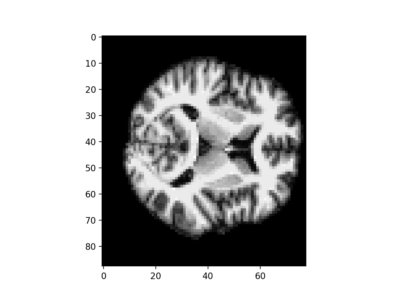
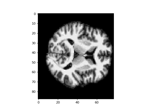
An example slice, over the third dimension:
>>> #: an example slice of skull-stripped structural
>>> plt.imshow(subject_data[:, :, 80])
<...>
The MNI template we want to match to is
mni_icbm152_t1_tal_nlin_asym_09a_masked_222.nii:
>>> #: the MNI template - also skull stripped
>>> template_img = nib.load('mni_icbm152_t1_tal_nlin_asym_09a_masked_222.nii')
>>> template_data = template_img.get_data()
>>> template_data.shape
(99, 117, 95)
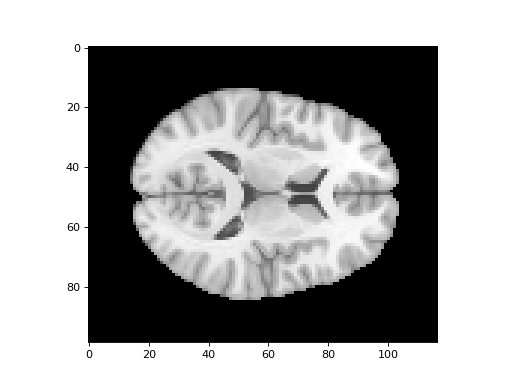
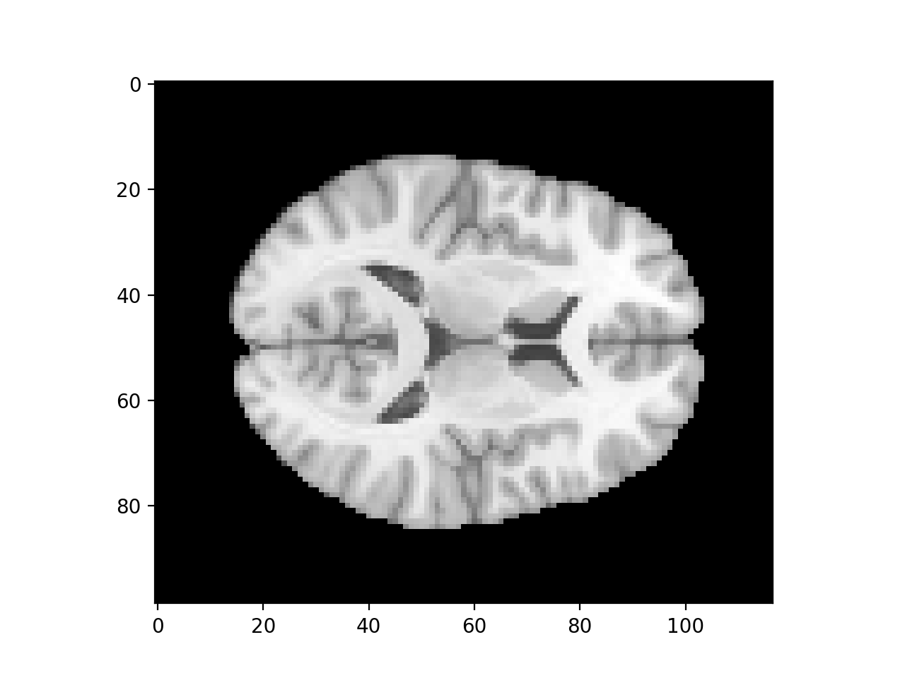
>>> #: example slice over the third dimension of the template
>>> plt.imshow(template_data[:, :, 42])
<...>

We have a current mapping from the voxels in the template image to the
voxels in the subject image, using the image affines. What is that mapping
(template_vox2subject_vox)?
>>> #- Get affine mapping from template voxels to subject voxels
Break up this affine into the 3 x 3 mat component and length 3 vec
translation component. We’ll need to use those in affine_transform:
>>> #- Break up `template_vox2subject_vox` into 3x3 `mat` and
>>> #- length 3 `vec`
Use scipy.ndimage.affine_transform to make a new version of the subject
image, resampled into the array size / shape of the template:
>>> #- Use affine_transform to make a copy of the subject image
>>> #- resampled into the array dimensions of the template image
>>> #- Call this resampled copy `subject_resampled`
>>> #- (we are going to use this array later).
>>> #- Use order=1 for the resampling (it is quicker)
Plot a slice from the resampled subject data next to the matching slice from
the template using subplots:
>>> #- Plot slice from resampled subject data next to slice
>>> #- from template data
Now we are going to try and do an affine match between these two images, using optimization.
We are going to need a cost function.
Remember, this takes the set of parameters we are using to transform the data, and returns a value that should be low when the images are well matched.
The value our cost function returns, is a mismatch metric.
I suggest you use the correlation mismatch function for the metric. Here is an implementation of the formula for the Pearson product-moment correlation coefficient:
where \(\bar{x}\) is the mean:
The correlation makes sense here, because both the subject scan and the template are T1-weighted images, meaning that we expect gray matter to be gray, white matter to be white, and CSF to be black. So, when the images are well-matched, the signal in one image should correlate highly with the signal from matching voxels in the other.
>>> #: the negative correlation mismatch metric
>>> def correl_mismatch(x, y):
...     """ Negative correlation between the two images, flattened to 1D
...     """
...     x_mean0 = x.ravel() - x.mean()
...     y_mean0 = y.ravel() - y.mean()
...     corr_top = x_mean0.dot(y_mean0)
...     corr_bottom = (np.sqrt(x_mean0.dot(x_mean0)) *
...                    np.sqrt(y_mean0.dot(y_mean0)))
...     return -corr_top / corr_bottom
Let’s check this gives the same answer as the standard numpy function. Here we are using Random numbers with np.random to give us samples from the standard normal distribution:
>>> #: check numpy agrees with our negative correlation calculation
>>> x = np.random.normal(size=(100,))
>>> y = np.random.normal(size=(100,))
>>> assert np.allclose(correl_mismatch(x, y), -np.corrcoef(x, y)[0, 1])
Now we need a function that will transform the subject image, given a set of transformation parameters.
Let’s use these transformation parameters:
x_t: translation in x;y_t: translation in y;z_t: translation in z;x_r: rotation around x axis;y_r: rotation around y axis;z_r: rotation around z axis;x_z: zoom (scaling) in x;y_z: zoom (scaling) in y;z_z: zoom (scaling) in z.
Say vol_arr is the image that we will transform.
Our function then returns a copy of vol_arr with those transformations
applied.
Let’s also say that these transformations are in millimeters (x, y, z coordinates).
That means we are going to make these transformations into a new 4 x 4 affine
P, and compose it with the template and subject affines:
- first - apply
template_vox2mmmapping to map to millimeters; - next - apply
Paffine made up of our transformations above; - next - apply
mm2subject_vox; - call the result
Q.
Finally, we want to apply the transformations in Q to make a resampled
copy of the subject image.
Our first task is to take the 9 parameters above, and return the affine matrix
P.
This function will look something like this:
def params2affine(params):
    # Unpack the parameter vector to individual parameters
    x_t, y_t, z_t, x_r, y_r, z_r, x_z, y_z, z_z = params
    # Matrix for zooms?
    # Matrix for rotations?
    # Vector for translations?
    # Build into affine
Hint: remember you have already imported x_rotmat etc from our
rotations module.
>>> #- Make params2affine function
>>> #- * accepts params vector
>>> #- * builds matrix for zooms
>>> #- * builds atrix for rotations
>>> #- * builds vector for translations
>>> #- * compile into affine and return
>>> #: some checks that the function does the right thing
>>> # Identity params gives identity affine
>>> assert np.allclose(params2affine([0, 0, 0, 0, 0, 0, 1, 1, 1]),
...                    np.eye(4))
>>> # Some zooms
>>> assert np.allclose(params2affine([0, 0, 0, 0, 0, 0, 2, 3, 4]),
...                    np.diag([2, 3, 4, 1]))
>>> # Some translations
>>> assert np.allclose(params2affine([0, 0, 0, 0, 0, 0, 2, 3, 4]),
...                    np.diag([2, 3, 4, 1]))
>>> # Some rotations
>>> assert np.allclose(params2affine([0, 0, 0, 0, 0, 0.2, 1, 1, 1]),
...                    [[np.cos(0.2), -np.sin(0.2), 0, 0],
...                     [np.sin(0.2), np.cos(0.2), 0, 0],
...                     [0, 0, 1, 0],
...                     [0, 0, 0, 1],
...                     ])
>>> assert np.allclose(params2affine([0, 0, 0, 0, 0, 0.2, 1, 1, 1]),
...                    [[np.cos(0.2), -np.sin(0.2), 0, 0],
...                     [np.sin(0.2), np.cos(0.2), 0, 0],
...                     [0, 0, 1, 0],
...                     [0, 0, 0, 1],
...                     ])
>>> assert np.allclose(params2affine([0, 0, 0, 0, -0.1, 0, 1, 1, 1]),
...                    [[np.cos(-0.1), 0, np.sin(-0.1), 0],
...                     [0, 1, 0, 0],
...                     [-np.sin(-0.1), 0, np.cos(-0.1), 0],
...                     [0, 0, 0, 1],
...                     ])
>>> assert np.allclose(params2affine([0, 0, 0, 0.3, 0, 0, 1, 1, 1]),
...                    [[1, 0, 0, 0],
...                     [0, np.cos(0.3), -np.sin(0.3), 0],
...                     [0, np.sin(0.3), np.cos(0.3), 0],
...                     [0, 0, 0, 1],
...                     ])
>>> # Translation
>>> assert np.allclose(params2affine([11, 12, 13, 0, 0, 0, 1, 1, 1]),
...                    [[1, 0, 0, 11],
...                     [0, 1, 0, 12],
...                     [0, 0, 1, 13],
...                     [0, 0, 0, 1]
...                     ])
Now we know how to make our affine P, we can make our cost function.
The cost function should accept the same vector of parameters as
params2affine, then:
- generate
P; - compose
template_vox2mm, thenPthenmm2subject_voxto giveQ; - resample the subject data using the matrix and vector from
Q(useorder=1resampling - it is quicker); - return the mismatch metric for the resampled image and template.
We can pick up the subject data and template data from the global namespace <global scope_>:
>>> #- Make a cost function called `cost_function` that will:
>>> #- * accept the vector of parameters containing x_t ... z_z
>>> #- * generate `P`;
>>> #- * compose template_vox2mm, then P then mm2subject_vox to give `Q`;
>>> #- * resample the subject data using the matrix and vector from `Q`.
>>> #-   Use `order=1` for the resampling - otherwise it will be slow.
>>> #- * return the mismatch metric for the resampled image and template.
>>> #: check the cost function returns the previous value if params
>>> # say to do no transformation
>>> current = correl_mismatch(subject_resampled, template_data)
>>> redone = cost_function([0, 0, 0, 0, 0, 0, 1, 1, 1])
>>> assert np.allclose(current, redone)
Now we are ready to optimize. We are going to need at least one of the cost
functions from scipy.optimize.
fmin_powell is a good place to start:
>>> #- get fmin_powell
Let’s define a callback so we can see what fmin_powell is doing:
>>> #: a callback we will pass to the fmin_powell function
>>> def my_callback(params):
...    print("Trying parameters " + str(params))
Now call fmin_powell with a starting guess for the parameters. Remember
to pass the callback with callback=my_callback.
This is going to take a crazy long time, dependingn on your computer. Maybe 10 minutes.
>>> #- Call optimizing function and collect best estimates for rotations
>>> #- Collect best estimates in `best_params` variable
Finally, use these parameters to:
- compile the P affine from the optimized parameters;
- compile the Q affine from the image affines and P;
- resample the subject image using the matrix and vector from this Q affine.
>>> #- * compile the P affine from the optimized parameters;
>>> #- * compile the Q affine from the image affines and P;
>>> #- * resample the subject image using the matrix and vector from the Q
>>> #-   affine.
Now you can look at the template and the resampled affine-normalized image side by side, using Subplots and axes in matplotlib:
>>> #- show example slice from template and normalized image