\(\newcommand{L}[1]{\| #1 \|}\newcommand{VL}[1]{\L{ \vec{#1} }}\newcommand{R}[1]{\operatorname{Re}\,(#1)}\newcommand{I}[1]{\operatorname{Im}\, (#1)}\)

Voxel time courses

When we have a 4D image, we can think of the data in several ways. For example the data could be:

• A series of 3D volumes (slicing over the last axis);
• A collection of 1D voxel time courses (slicing over the first three axes).

>>> # Our usual set-up
>>> import numpy as np
>>> import matplotlib.pyplot as plt
>>> # Display array values to 4 digits of precision
>>> np.set_printoptions(precision=4, suppress=True)

We load a 4D file:

>>> import nibabel as nib
>>> img = nib.load('ds114_sub009_t2r1.nii')
>>> img.shape
(64, 64, 30, 173)

We drop the first volume; as you remember, the first volume is very different from the rest of the volumes in the series:

>>> # Drop the first volume
>>> data = img.get_data()
>>> data = data[..., 1:]
>>> data.shape
(64, 64, 30, 172)

We can think of this 4D data as a series of 3D volumes. That is the way we have been thinking of the 4D data so far:

>>> # This is slicing over the last (time) axis
>>> vol0 = data[..., 0]
>>> vol0.shape
(64, 64, 30)

We can also index over the first three axes. The first three axes in this array represent space.

• The first axis goes from right to left (0 index value means right, 63 means left);
• The second axis goes from back to front (0 index value means back, 63 means front);
• The third axes goes from bottom to top (0 means bottom, 29 means top).

If you give me index values for these first three axes, you have given me a coordinate in the first three axes of the array.

For example, you could give me an index tuple for the first three axes like this: (42, 32, 19). The first index of 42 refers to a position towards the left of the brain (> 31). The second index of 32 refers to a position almost in the center front to back. The last index of 19 refers to a position a little further towards the top of the brain – in this image.

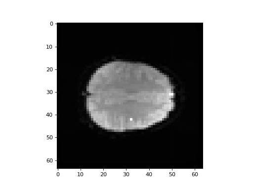
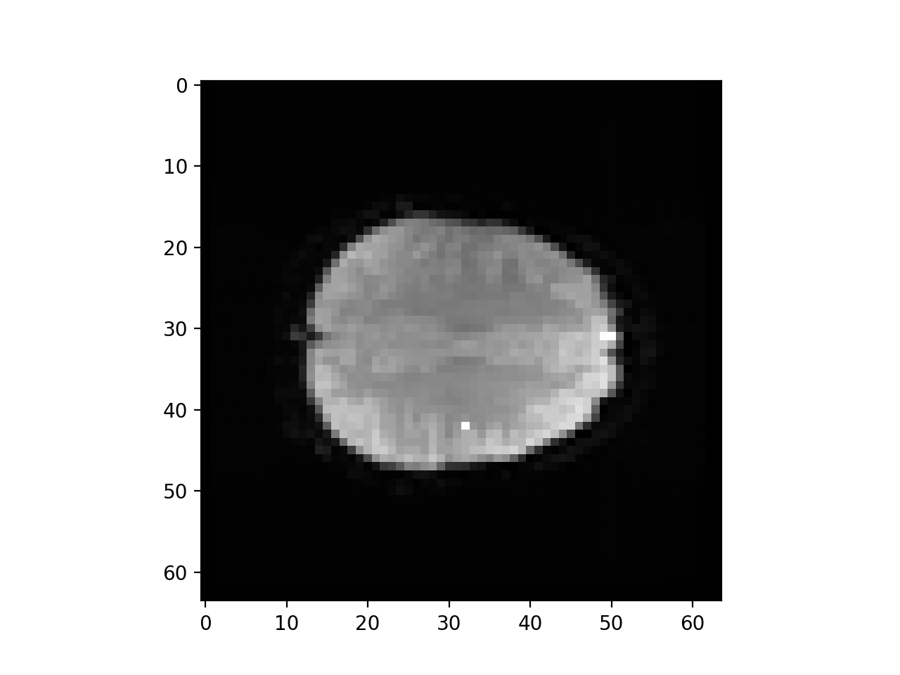
This coordinate therefore refers to a particular part of the image:

>>> # Where is this in the brain?
>>> mean_data = np.mean(data, axis=-1)
>>> # Make a nice bright dot in the right place
>>> mean_data[42, 32, 19] = np.max(mean_data)
>>> plt.imshow(mean_data[:, :, 19], cmap='gray', interpolation='nearest')
<...>

(png, hires.png, pdf)

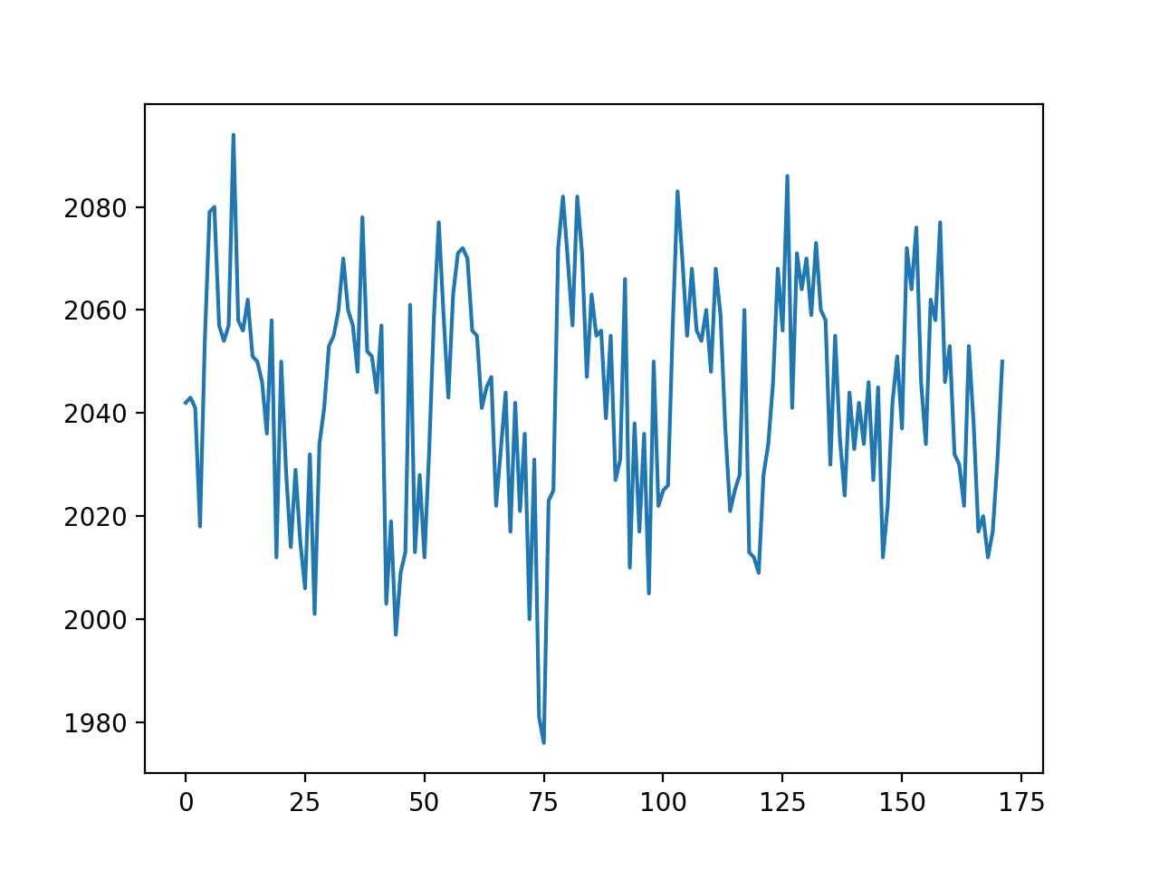
If I slice into the data array with these coordinates, I will get a vector, with the image value at that position (43, 32, 19), for every point in time:

>>> # This is slicing over all three of the space axes
>>> voxel_time_course = data[42, 32, 19]
>>> voxel_time_course.shape
(172,)
>>> plt.plot(voxel_time_course)
[...]

(png, hires.png, pdf)

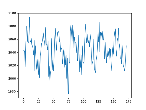
We could call this a “voxel time course”.

We might want to do ordinary statistical type things with this time course. For example, we might want to correlate this time course with a measure of whether the subject was doing the task or not.

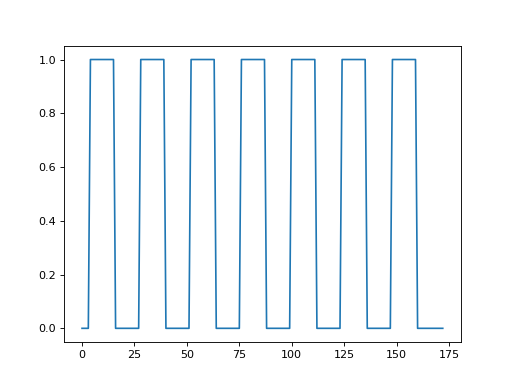
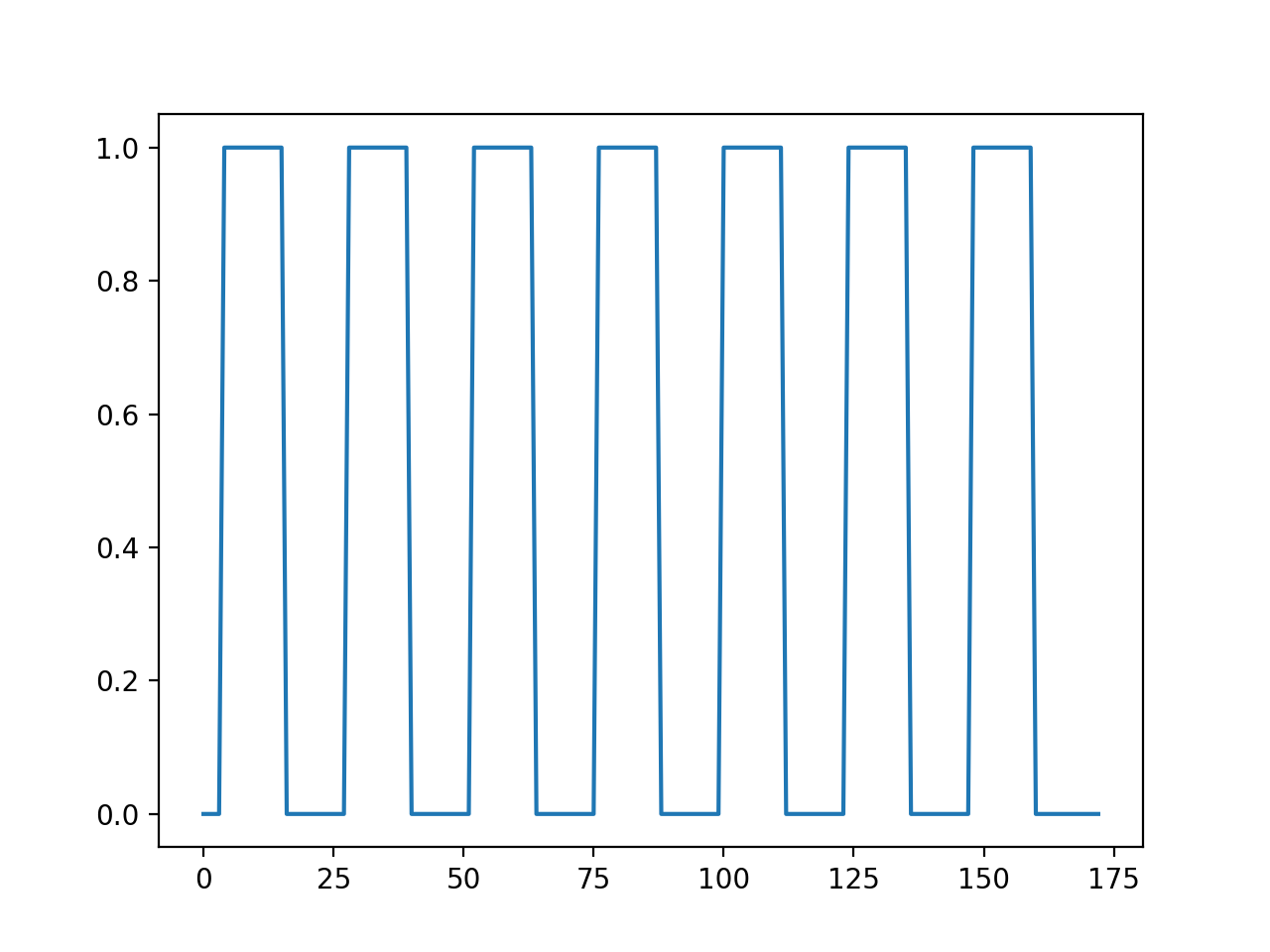
This measure will have 1 for each volume (time point) where the subject was doing the task, and 0 for each volume where the subject was at rest.

We call this a “neural” time course, because we believe that the nerves in the relevant brain area will switch on when the task starts (value = 1) and then switch off when the task stops (value = 0).

To get this on-off measure, we will use our pre-packaged function for OpenFMRI data:

>>> # Load the neural time course using pre-packaged function
>>> from stimuli import events2neural
>>> TR = 2.5  # time between volumes
>>> n_trs = img.shape[-1]  # The original number of TRs
>>> neural = events2neural('ds114_sub009_t2r1_cond.txt', TR, n_trs)
>>> plt.plot(neural)
[...]

(png, hires.png, pdf)

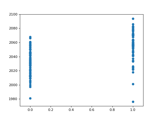
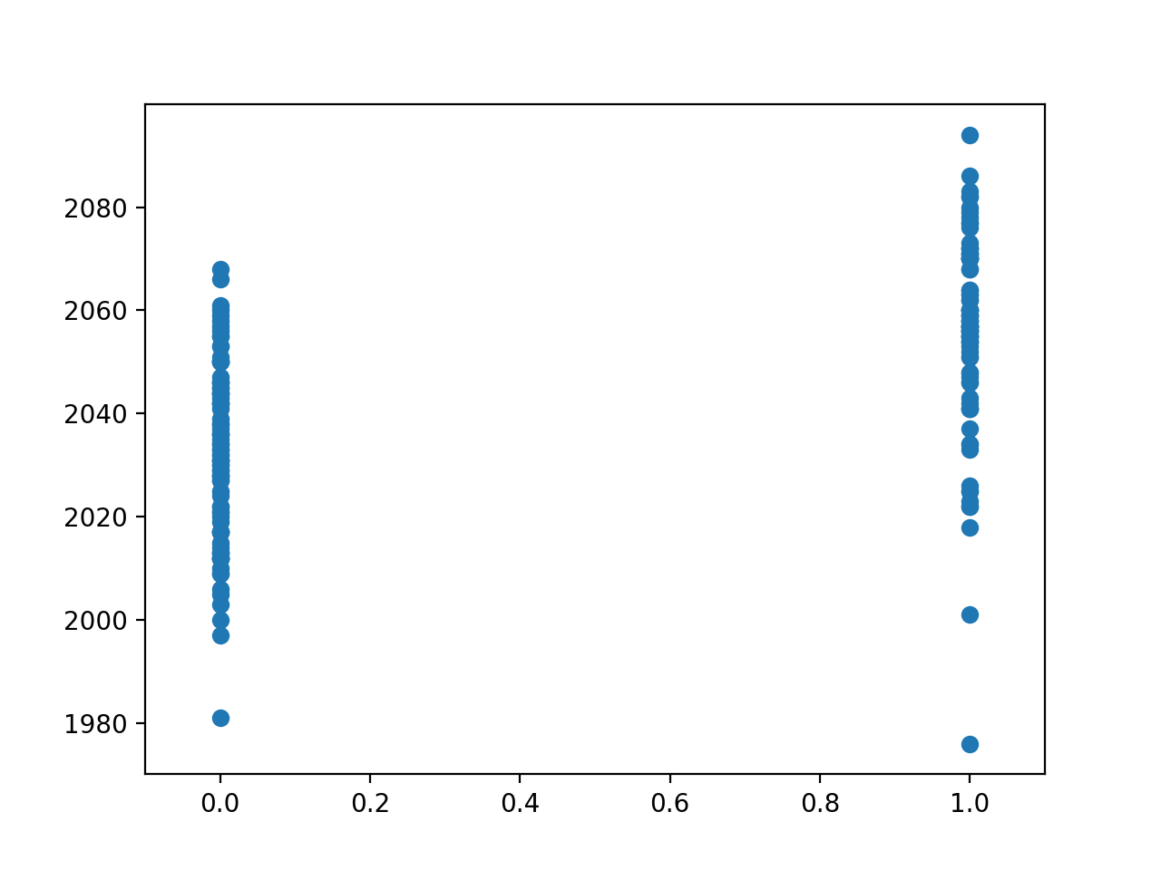
Here we plot the voxel time course against this neural prediction:

>>> # Plot the neural prediction against the data
>>> neural = neural[1:]
>>> # Notice the 'o' to specify the "line marker"
>>> plt.plot(neural, voxel_time_course, 'o')
[...]
>>> # Set the axis limits to give space on left and right
>>> axis = plt.gca()
>>> axis.set_xlim(-0.1, 1.1)
(...)

(png, hires.png, pdf)

We can look at the correlation between the on-off prediction and the voxel time course:

>>> # Correlate the neural time course with the voxel time course
>>> np.corrcoef(neural, voxel_time_course)
array([[ 1.    ,  0.5429],
       [ 0.5429,  1.    ]])