\(\newcommand{L}[1]{\| #1 \|}\newcommand{VL}[1]{\L{ \vec{#1} }}\newcommand{R}[1]{\operatorname{Re}\,(#1)}\newcommand{I}[1]{\operatorname{Im}\, (#1)}\)

Applying deformations exercise

Requirements:

• Removing length 1 axes with numpy.squeeze;
• numpy.tranpose for swapping axes;
• Resampling with scipy.ndimage;
• The nibabel.affines module;
• General resampling between images with scipy.ndimage.map_coordinates.

>>> #: standard imports
>>> import numpy as np
>>> import matplotlib.pyplot as plt
>>> # print arrays to 4 decimal places
>>> np.set_printoptions(precision=4, suppress=True)
>>> import numpy.linalg as npl
>>> import nibabel as nib

>>> #: gray colormap and nearest neighbor interpolation by default
>>> plt.rcParams['image.cmap'] = 'gray'
>>> plt.rcParams['image.interpolation'] = 'nearest'

Applying a deformation field

We should have already calculated the deformation field for the image ds107_sub012_highres.nii.

We did this using the SPM12 Normalise: Estimate option from the GUI.

This should have left an image called y_ds107_sub012_highres.nii in your working directory.

If not:

• Ask for help;
• If you get stuck, you can download the image from y_ds107_sub012_highres.nii.

We make an image object for this deformations image by loading with nibabel.

>>> #: load y_ds107_sub012_highres.nii with nibabel
>>> # get the image array data
>>> deformations_img = nib.load('y_ds107_sub012_highres.nii')
>>> deformations_data = deformations_img.get_data()
>>> deformations_data.shape
(121, 145, 121, 1, 3)

We are going to work out how to apply this deformations image to reslice our original image ds107_sub012_highres.nii.

Oddly - this is a 5 dimensional image, where the 4th dimension is length 1.

The length-1 4th dimension is an artefact of the NIfTI image format – so let’s get rid of this dimension with np.squeeze:

>>> #: remove length-1 4th dimension from deformation data
>>> deformations_data = np.squeeze(deformations_data)
>>> deformations_data.shape
(121, 145, 121, 3)

The data is now a 4-dimensional image, containing 3 volumes. These volumes are:

• x coordinates;
• y coordinates;
• z coordinates

respectively.

Put another way, the vector deformations_data[i, j, k, :] gives the (x, y, z) coordinates for the voxel [i, j, k]. More on this later.

If you were looking carefully at the SPM interface, SPM has calculated the distortions necessary to go from a template of tissue probability maps (called TPM.nii) to the ds107_sub012_highres.nii image.

We can get the original 3D shape and affine of TPM.nii because SPM stored them in y_ds107_sub012_highres.nii:

>>> #: get original TPM.nii 3D shape and affine
>>> tpm_shape = deformations_data.shape[:3]
>>> tpm_affine = deformations_img.affine
>>> tpm_affine
array([[  -1.5,    0. ,    0. ,   90. ],
       [   0. ,    1.5,    0. , -126. ],
       [   0. ,    0. ,    1.5,  -72. ],
       [   0. ,    0. ,    0. ,    1. ]])

First we look at the images before the normalization has been applied.

To do that, we will make a new copy of the MNI template, with the same shape as the TPM image.

The MNI template image we will use is mni_icbm152_t1_tal_nlin_asym_09a.nii.

>>> #: load the template image we will resample from
>>> template_img = nib.load('mni_icbm152_t1_tal_nlin_asym_09a.nii')
>>> template_data = template_img.get_data()
>>> template_data.shape
(197, 233, 189)

Now we need the mapping from voxels in TPM.nii to voxels in mni_icbm152_t1_tal_nlin_asym_09a.nii.

We can break this down into two transforms:

• from voxels in TPM.nii to (x, y, z) mm;
• from (x, y, z) mm to voxels in mni_icbm152_t1_tal_nlin_asym_09a.nii.

We have these transforms already. The full transform is:

>>> #: voxels in TPM.nii to voxels in mni_icbm152_t1_tal_nlin_asym_09a.nii
>>> # Matrix multiplication is right to left
>>> vox2vox = npl.inv(template_img.affine).dot(tpm_affine)
>>> vox2vox
array([[  -1.5,    0. ,    0. ,  188. ],
       [   0. ,    1.5,    0. ,    8. ],
       [   0. ,    0. ,    1.5,    0. ],
       [   0. ,    0. ,    0. ,    1. ]])

We break this down into the 3 x 3 mat and length 3 vec components:

>>> #: to mat and vec
>>> mat, vec = nib.affines.to_matvec(vox2vox)
>>> mat
array([[-1.5,  0. ,  0. ],
       [ 0. ,  1.5,  0. ],
       [ 0. ,  0. ,  1.5]])
>>> vec
array([ 188.,    8.,    0.])

Then we resample from the MNI template, into the voxel grid of the TPM.nii:

>>> #: resample MNI template onto TPM grid
>>> from scipy.ndimage import affine_transform
>>> template_into_tpm = affine_transform(template_data, mat, vec,
...                                      output_shape=tpm_shape)
>>> template_into_tpm.shape
(121, 145, 121)

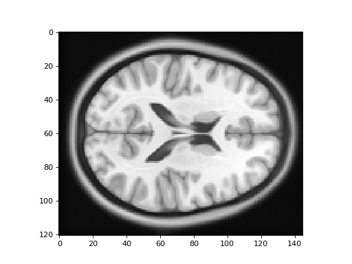
Here is the new version of the template image:

>>> #: plot the template image resampled onto the TPM grid
>>> plt.imshow(template_into_tpm[:, :, 60])
<...>

(png, hires.png, pdf)

Now, what to do with with the SPM distortion field in deformations_data?

By checking in the SPM source code [1], it is possible to work out that deformations_data contains, for every voxel in TPM, the corresponding mm coordinate in the mm space of the subject image.

That is, deformations_data[i, j, k] is a length 3 vector [x, y, z] where [x, y, z] are the mm coordinates of voxel [i, j, k] when mapped into millimeters for the subject image.

Here is the subject data, and the image, which contains the affine:

>>> #: load the subject data that we will resample from
>>> subject_img = nib.load('ds107_sub012_highres.nii')
>>> subject_data = subject_img.get_data()
>>> subject_data.shape
(256, 208, 192)

With this information, and with the scipy.ndimage.map_coordinates function, you should be able to:

• get the mapping from voxels in TPM to voxels in the subject image and;
• resample the subject image into the grid of the TPM image using this mapping.

Hint: remember that map_coordinates expects the 3-length coordinate dimension to be first, but deformations_data – at the moment – has the 3-length coordinate dimension last.

>>> #- * get mapping from voxels in TPM to voxels in the subject image;
>>> #- * resample the subject image into the grid of the TPM image using
>>> #-   this mapping.
>>> from scipy.ndimage import map_coordinates
>>> vox2vox_mapping = nib.affines.apply_affine(npl.inv(subject_img.affine), deformations_data)
>>> for_map_coords = vox2vox_mapping.transpose(3, 0, 1, 2)
>>> subject_into_tpm = map_coordinates(subject_data, for_map_coords)
>>> subject_into_tpm.shape
(121, 145, 121)

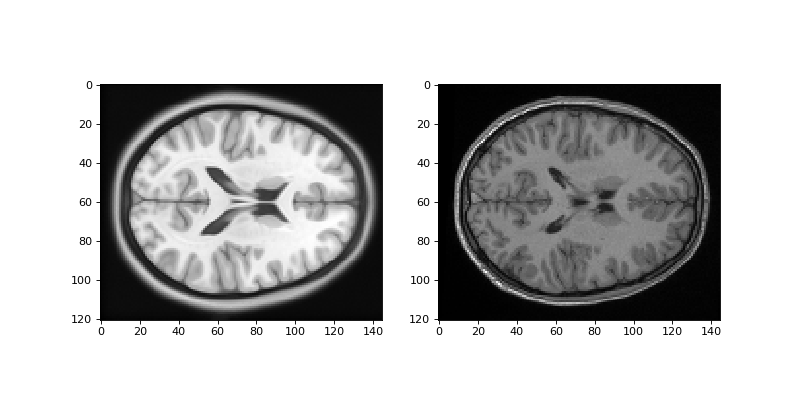
Show an example slice from the template resampled into the TPM voxel grid, and the subject resampled into the TPM voxel grid:

>>> #- show an example slice from the resampled template and resampled
>>> #- subject
>>> fig, axes = plt.subplots(1, 2, figsize=(10, 5))
>>> axes[0].imshow(template_into_tpm[:, :, 60])
<...>
>>> axes[1].imshow(subject_into_tpm[:, :, 60])
<...>

(png, hires.png, pdf)

Footnotes

[1]

It’s not very easy to work through the SPM12 source code for this, but if you want to check for yourself, you’ll find that the SPM batch interface for “Normalise: Write” is in config/spm_run_norm.m. The batch interface calls the sub-function norm_write. norm_write collects the NIfTI file with the y_ prefix that contains the deformations, if the user did not specify the file, and calls the spm_deformations function. This function in turn calls down into the pull_def sub-function, in which SPM calculates the matrix Y, which is the (I, J, K, 3) image data from the deformations NIfTI file, left multiplied by the mm to voxel mapping for the image being resampled. pull_def then resamples from the image to which we are applying “Normalize: Write”, using the Y array as voxel coordinates. Therefore the y_-prefixed deformation field image contains the coodinates mapping from voxels in the template to millimeters in the image that was registered.